Self-Attention Mechanism

This post covers the idea behind Self-Attention Mechanism, explaining step-by-step how it works in the Transformer architecture.

Table of contents

Motivation Example of Self-Attention

Consider these sentences:

• America shrew mole.
• One mole of CO2 weighs 44 grams.

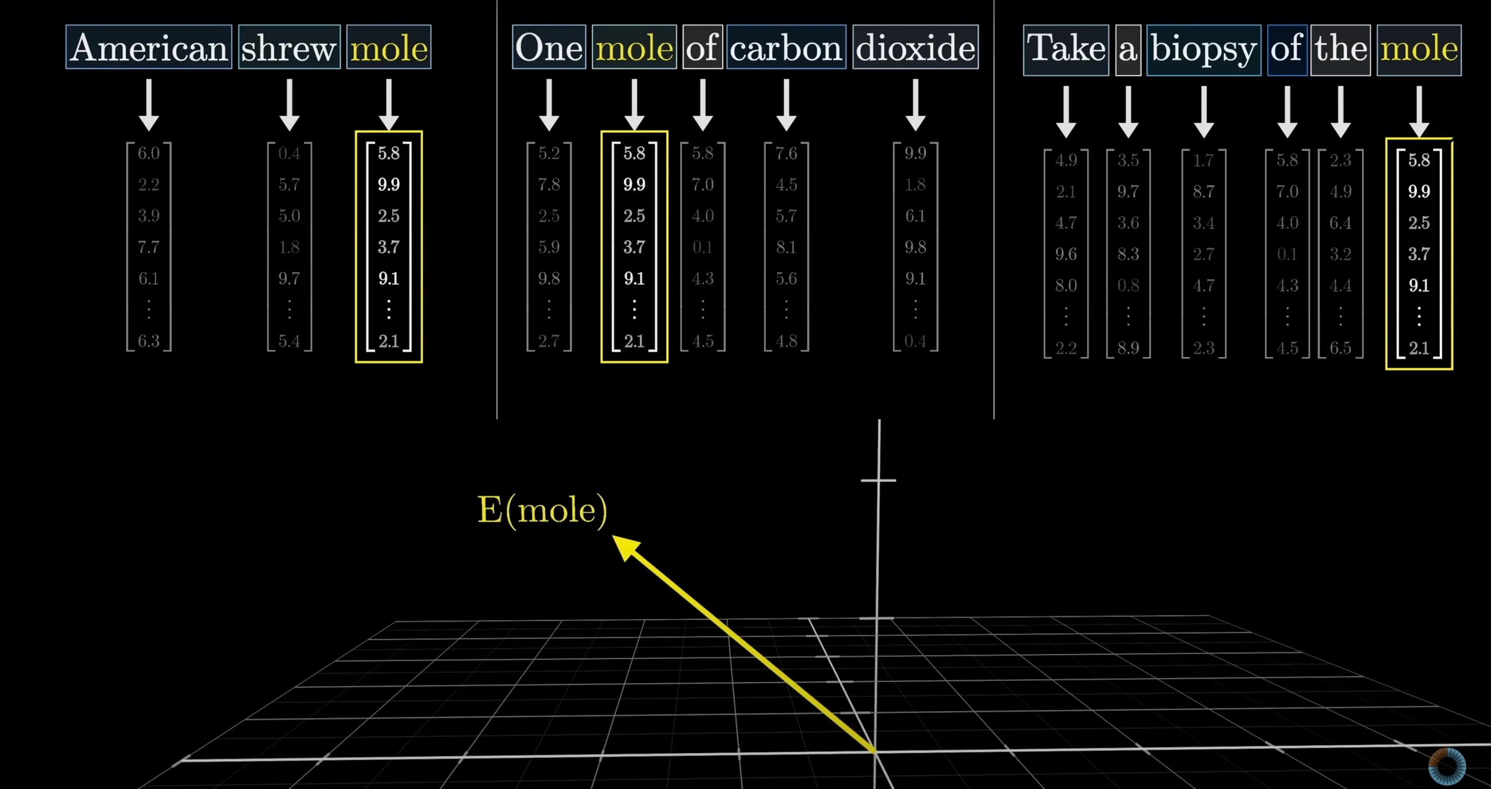Figure 1: The word “mole” carries completely different semantic meanings depending on the surrounding context.

You can see that the word “mole” has different meanings in these two sentences, based on the sentence context.

However, in a traditional RNN or static embedding model, after the initial embedding step, each token is associated with a fixed vector representation. So in this case, the word “mole” would start with the exact same initial vector representation regardless of surrounding context.

How Transformers Predict the Next Word: Context Aggregation

In an autoregressive Transformer (such as GPT), the model generates text token-by-token by predicting the next word given a sequence of prompt tokens.

To predict what word comes next after a prompt sequence (for example, “Therefore, the murderer was…”):

It will have to have somehow encoded all of the information from the full context window that’s relevant to predicting the next word into the vector representation of the final word.

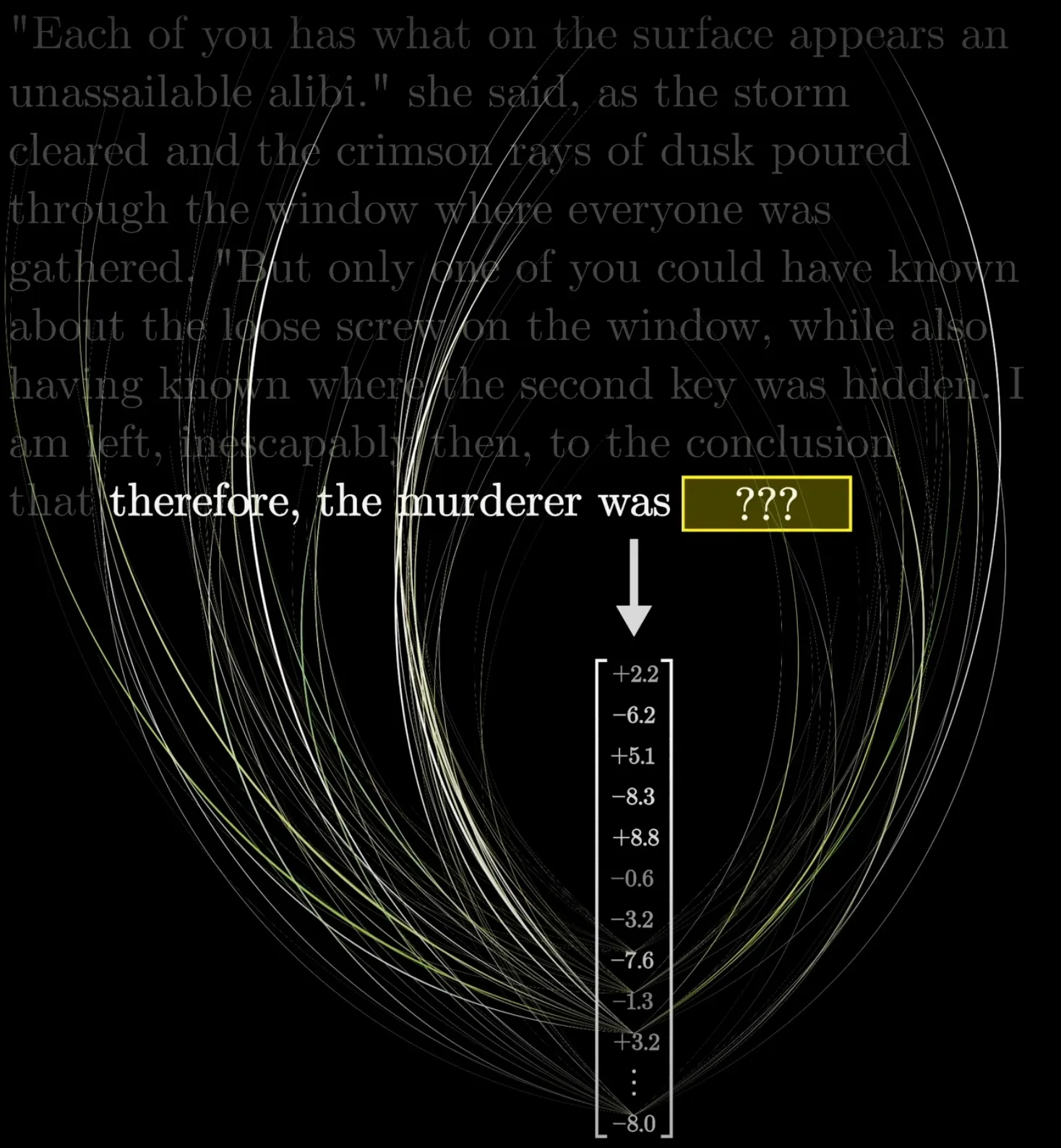Figure 2: The final vector embedding (e.g., for “was”) ingests and encodes all relevant context from preceding tokens across the full context window to predict the next word.

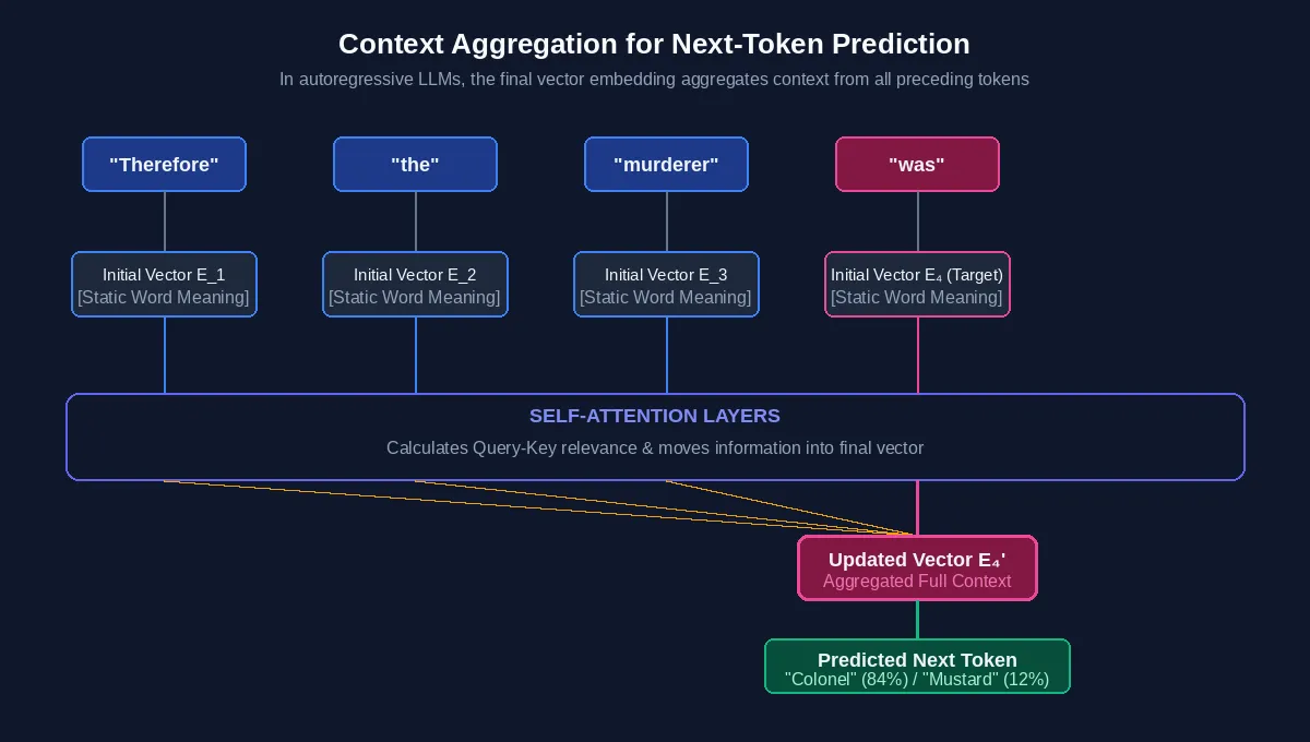Figure 3: Information flow diagram in a Transformer context window. Self-attention passes information from preceding token vectors into the final token vector ($\vec{E}_4 \to \vec{E}_4'$) to enable next-token prediction.

1. Initial Embeddings ($\vec{E}_i$): Each token in the context window begins as a static vector lookup ($\vec{E}_1, \vec{E}_2, \vec{E}_3, \vec{E}_4$).
2. Context Aggregation via Attention: The model does not generate predictions from every position. Instead, the final token vector (at position $N$, here "was") must ingest, filter, and aggregate key clues from all preceding tokens.
3. Vector Transformation ($\vec{E}_4 \to \vec{E}_4'$): Through multiple layers of Self-Attention, information from previous token vectors is moved into the final token’s vector representation.
4. Final Prediction: The enriched vector $\vec{E}_4'$ is passed through the model’s final output projection layer (Unembedding / Softmax) to compute probability scores for the next token (e.g., "Colonel" or "Mustard").

The Attention Pattern

We’ll begin by describing a single head of attention, and later we will see how attention with multiple heads run in parallel.

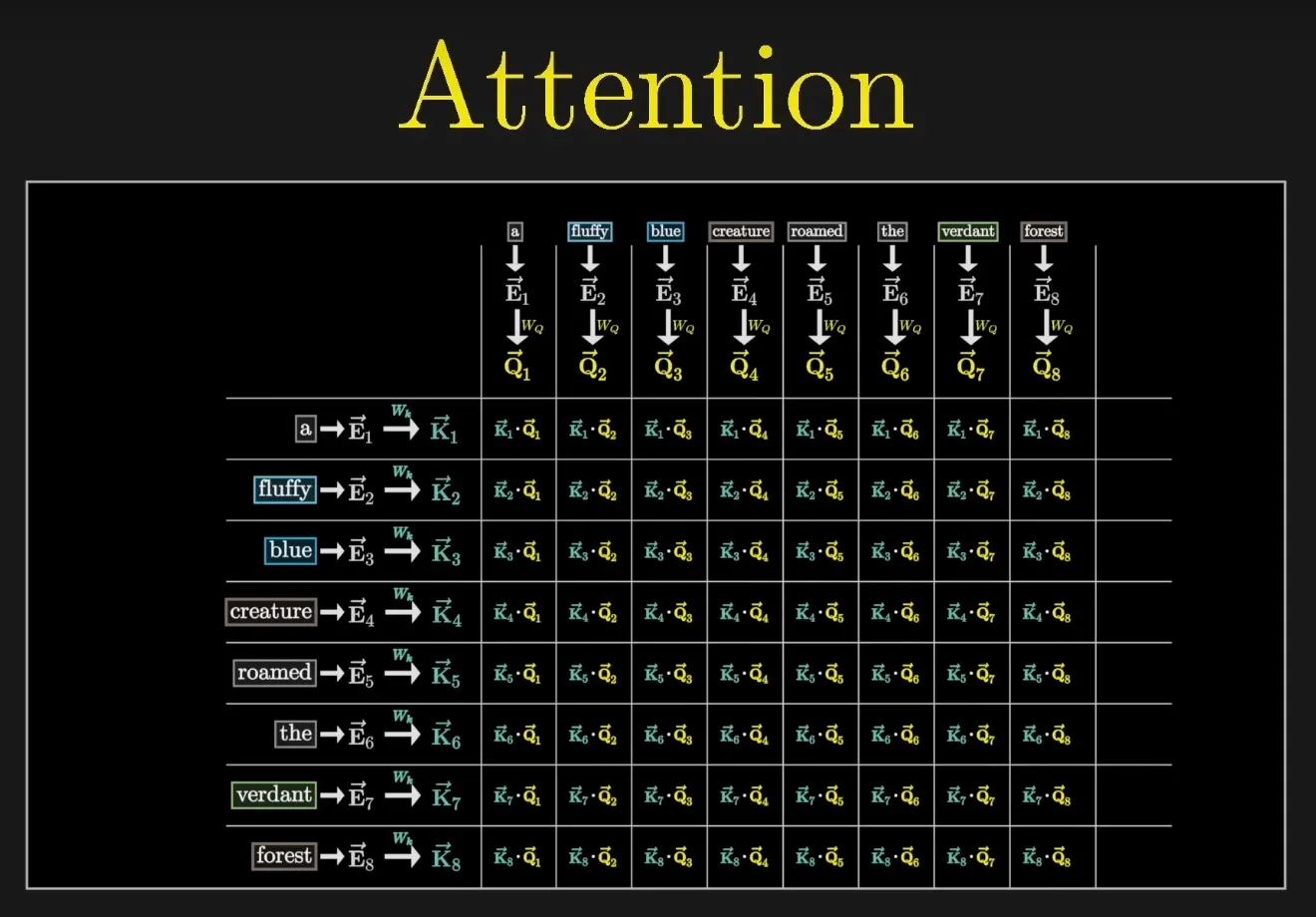Figure 4: The structure of a Single-Head Self-Attention block. Each token embedding is projected into Queries, Keys, and Values to calculate attention scores and update token representations.

The QKV Mechanism: Queries, Keys, and Values

To allow token vectors to exchange context, Self-Attention transforms each initial embedding vector into three specialized role vectors:

• Query ($Q$): “What am I looking for?”
• Key ($K$): “What information do I contain?”
• Value ($V$): “What content do I transfer if matched?”

Deep Dive: Query Vectors ($Q$)

A Query vector ($\vec{Q}_i$) represents the questions or requirements a specific token $i$ broadcasts to other tokens in the context window.

1. Calculation via Linear Projection

For each token embedding $\vec{E}_i$, its Query vector $\vec{Q}_i$ is computed by multiplying with a learned linear projection matrix $W_Q$:

$\vec{Q}_i = W_Q \vec{E}_i$

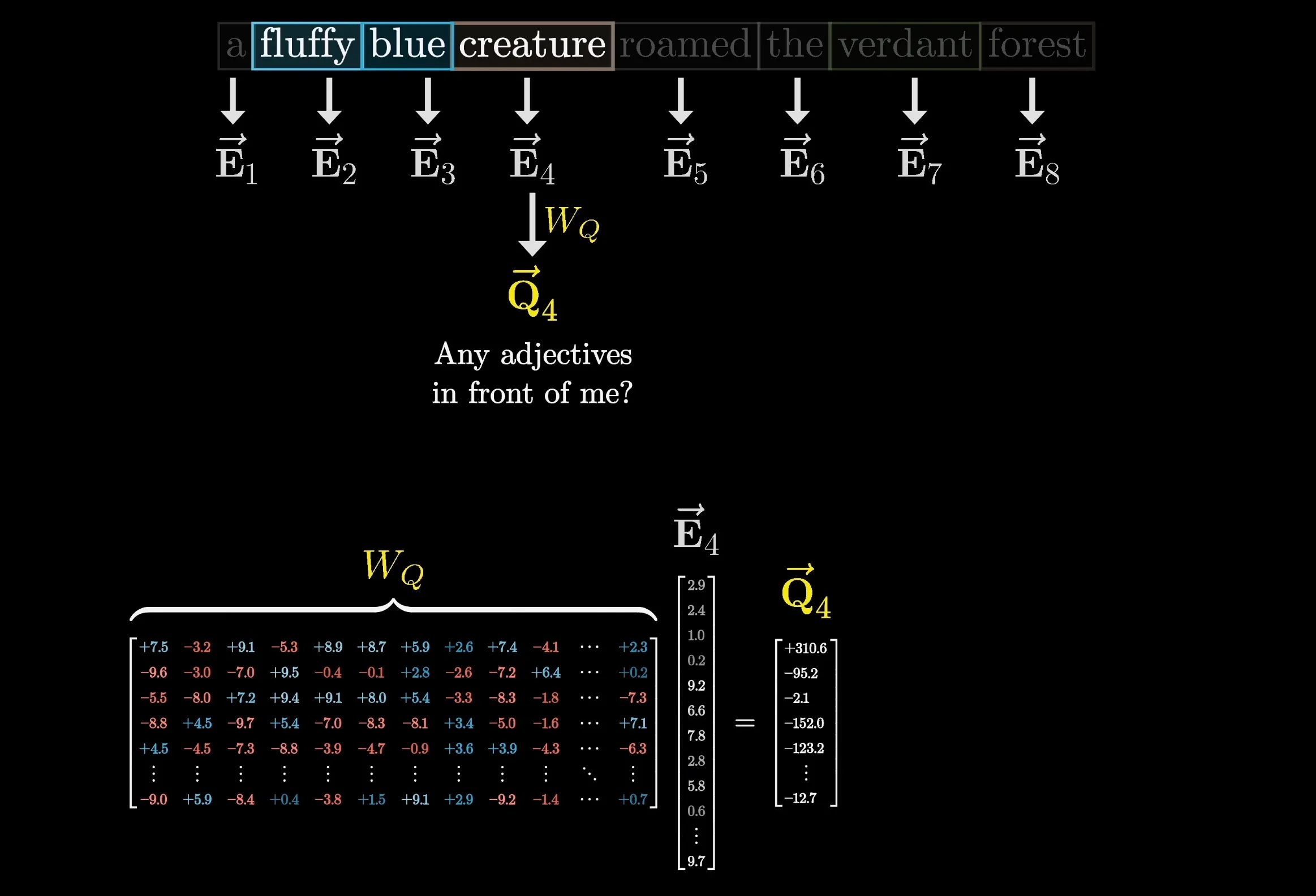Figure 5: Computing the Query vector $\vec{Q}_4$ for the token “creature” by multiplying its embedding $\vec{E}_4$ by the learned weight matrix $W_Q$. The resulting vector asks: “Any adjectives in front of me?“

2. Parallel Computation Across All Tokens

Every token embedding in the sequence is multiplied by the same weight matrix $W_Q$ simultaneously:

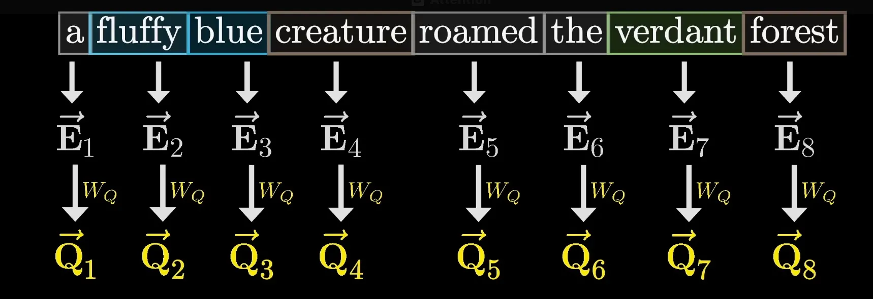Figure 6: Each token’s initial embedding $\vec{E}_i$ is projected by $W_Q$ into its corresponding Query vector $\vec{Q}_i$ in parallel.

3. What Does a Query Do?

In high-dimensional space, the Query vector encodes specific semantic questions:

• For a noun like “creature”: Its Query asks, “Are there adjectives preceding me that describe my appearance?”
• For an ambiguous noun like “mole”: Its Query asks, “Is there context showing whether I am an animal or a chemistry unit?”
• For a verb like “was”: Its Query asks, “Who or what is the subject of this clause?”

Deep Dive: Key Vectors ($K$)

While a Query vector asks a question, a Key vector ($\vec{K}_j$) advertises what information a token holds to answer potential queries.

1. Calculation via Linear Projection

Just like Queries, Key vectors are computed by multiplying each token embedding by a separate learned weight matrix $W_K$:

$\vec{K}_j = W_K \vec{E}_j$

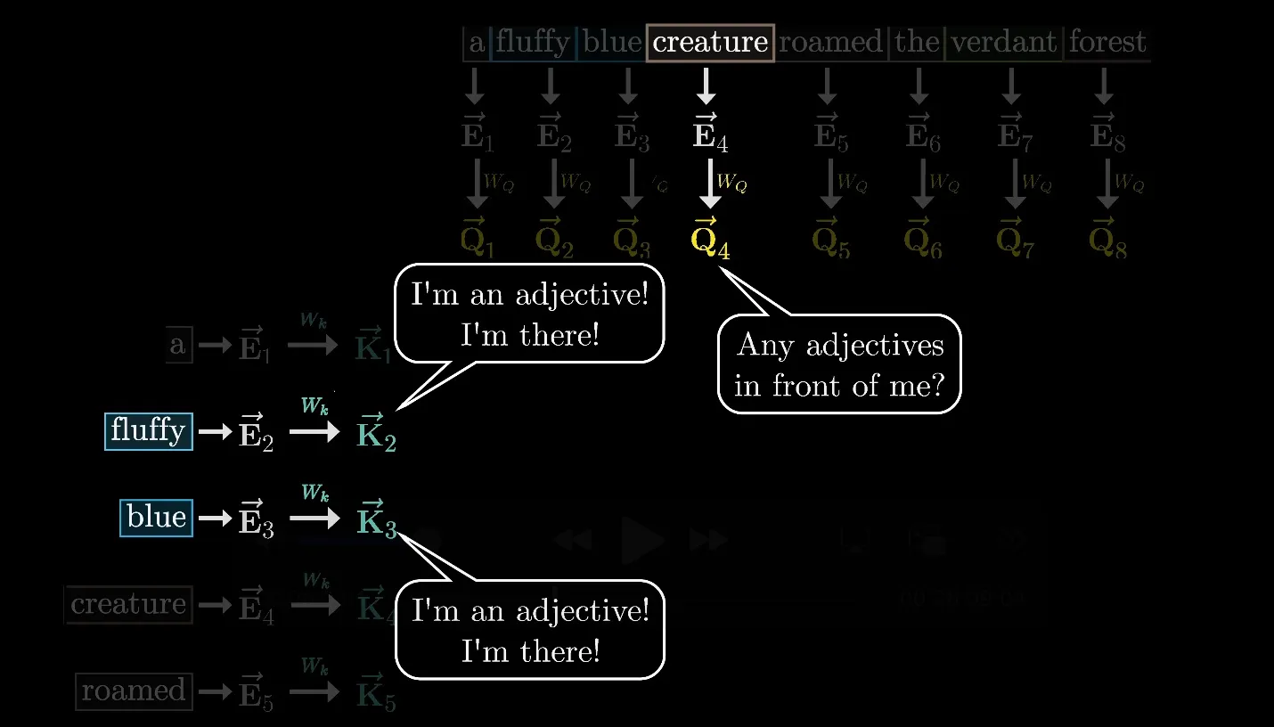Figure 7: Token embeddings are projected by $W_K$ into Key vectors $\vec{K}_j$. When $\vec{Q}_4$ (“creature”) asks for adjectives, the keys for “fluffy” ($\vec{K}_2$) and “blue” ($\vec{K}_3$) respond: “I’m an adjective! I’m there!“.

2. Matching Queries and Keys (Dot Product)

To determine how relevant token $j$ is to token $i$, the model computes the dot product between Query $\vec{Q}_i$ and Key $\vec{K}_j$:

$\text{Score}_{ij} = \vec{K}_j \cdot \vec{Q}_i$

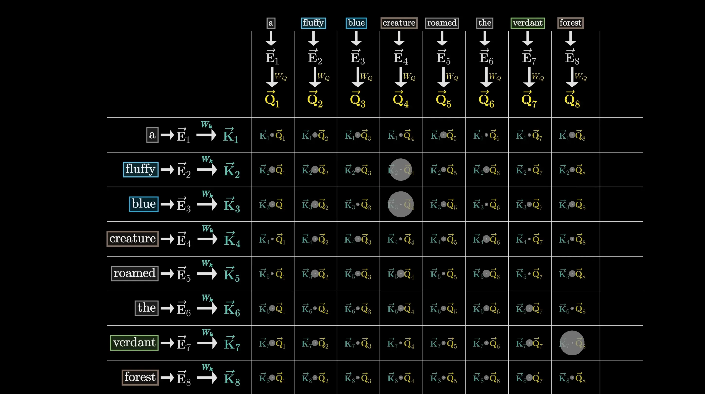Figure 8: Dot product grid between all Keys ($\vec{K}_1 \dots \vec{K}_8$) and Queries ($\vec{Q}_1 \dots \vec{Q}_8$). Highlighted cells show strong alignment where Keys answer Queries—such as $\vec{K}_2$ (“fluffy”) and $\vec{K}_3$ (“blue”) strongly matching $\vec{Q}_4$ (“creature”).

• Geometric Meaning: The dot product measures vector alignment. When a Query and a Key point in similar directions in embedding space, their dot product is large and positive.
• High Positive Score: The Key matches the Query (e.g., $\vec{K}_{\text{fluffy}} \cdot \vec{Q}_{\text{creature}}$). Strong affinity indicates contextual information should transfer.
• Low or Negative Score: The Key is irrelevant or orthogonal to the Query. Little to no information will transfer.

Value Vectors

After computing all the dot products of the key-query pairs, we get the grid with values ranging from $-\infty$ to $\infty$, which displays the relevance between words.

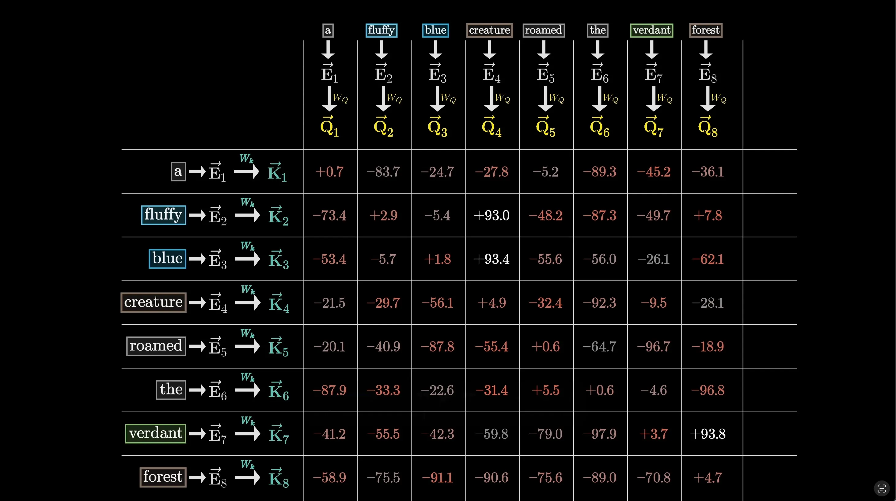Figure 9: The raw dot-product score grid computed for all Key-Query pairs, showing relevance scores ranging from $-\infty$ to $\infty$.

The way we’re about to use these scores is by taking a certain value along each column with most relevance.

But first, instead of having values between $-\infty$ and $\infty$, we want the values to be between $0$ and $1$ so they can be a probability distribution.

If you are coming from the last chapter, you may be familiar with softmax, which is really useful in this case to normalize the values.

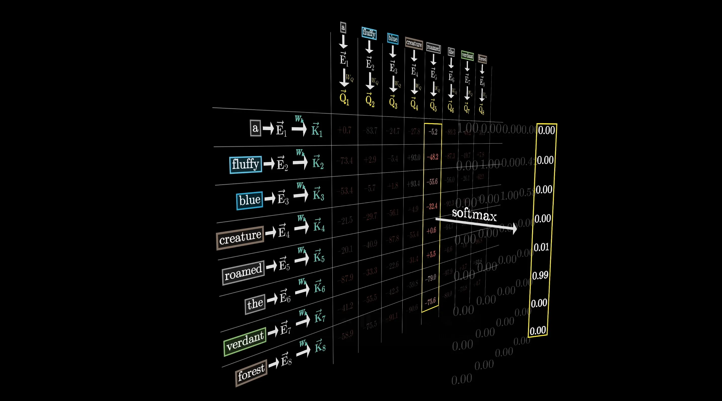Figure 10: Applying softmax down each column to normalize scores into a valid probability distribution.

After we apply softmax to all the columns, we will get the grid with these normalized values, and we call this grid the Attention Pattern.

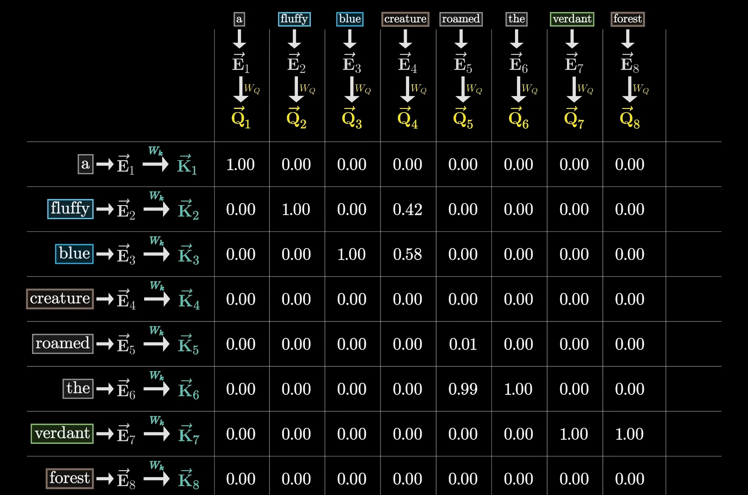Figure 11: The Attention Pattern grid after applying softmax column-by-column.

The original transformer paper presents us with a really compacted way to write this down (The Attention Formula):

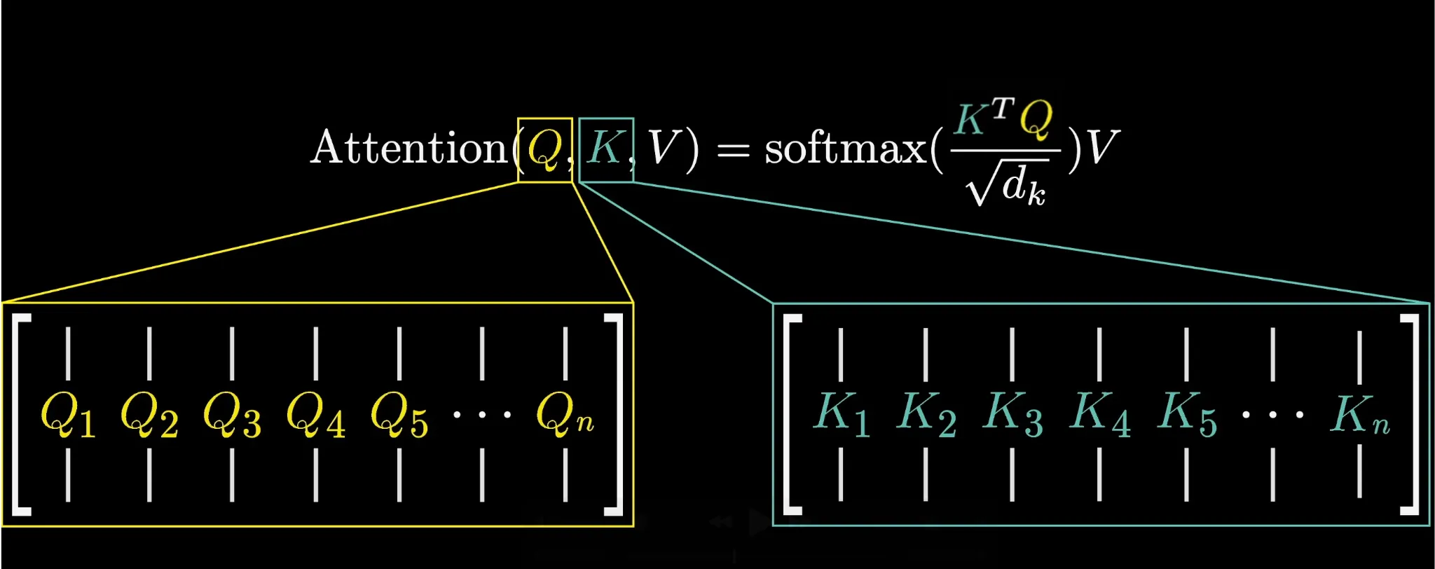Figure 12: The Attention Formula from the original Transformer paper (“Attention Is All You Need”).

A small notice is that for numerical stability, it’s helpful to divide these values by the square root of the dimension of key-query space ($\sqrt{d_k}$).

Finally, I have cover the formula for attention pattern but what is the last factor in the formula. As for the $V$ term, I will explain about it in just a second.

In earlier blog, I have shown that during the training process, the model is run on a given text example, guess the next word. Then the model will adjust the weights based on the probability assigns to the true next word.

But in real word, there is actually more to this. It turns out that in order to make the process more efficient, the model also simultaneously predicts every next token during a sentence. It runs in parallel the sentences as below:

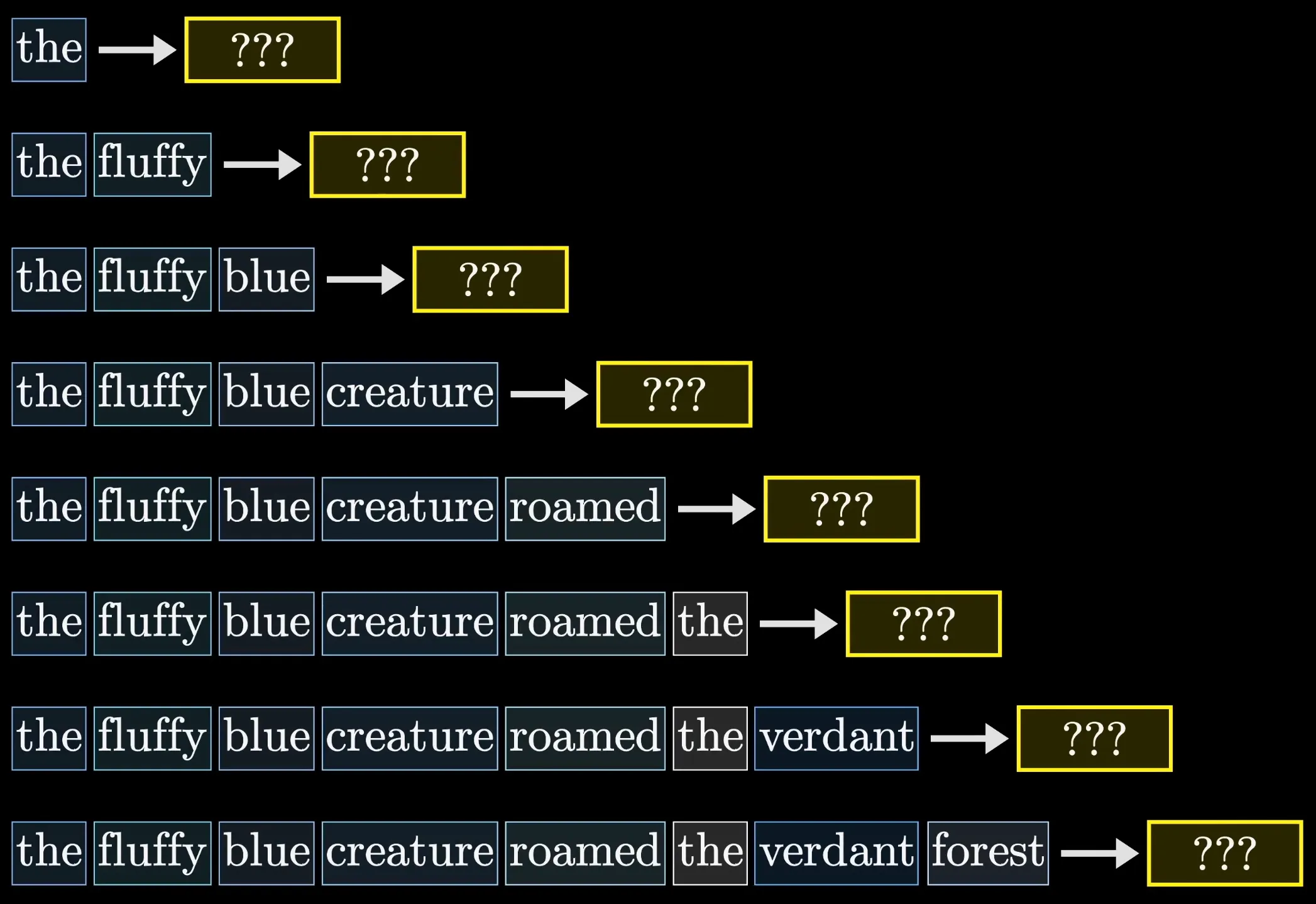Figure 13: The model simultaneously predicts every subsequent token in parallel during training.

This makes the training process become more efficient.

However, there is a problem that the model can look at the words that appear later can be influence to the words that appear earlier since these sentences are running simultaneously. This is just like a student doing the examination with direct answers next to it.

In order to prevent this, what we currently do is to force the spots where later token have influence on the earlier token somehow become zero. A common way to do this is that prior to applying softmax, we set all the value in Attention Pattern Grid with those entries become negative infinity ($-\infty$). This will make the softmax value become zero and thus the later token will not have any influence on the earlier token.

This process is called masking.

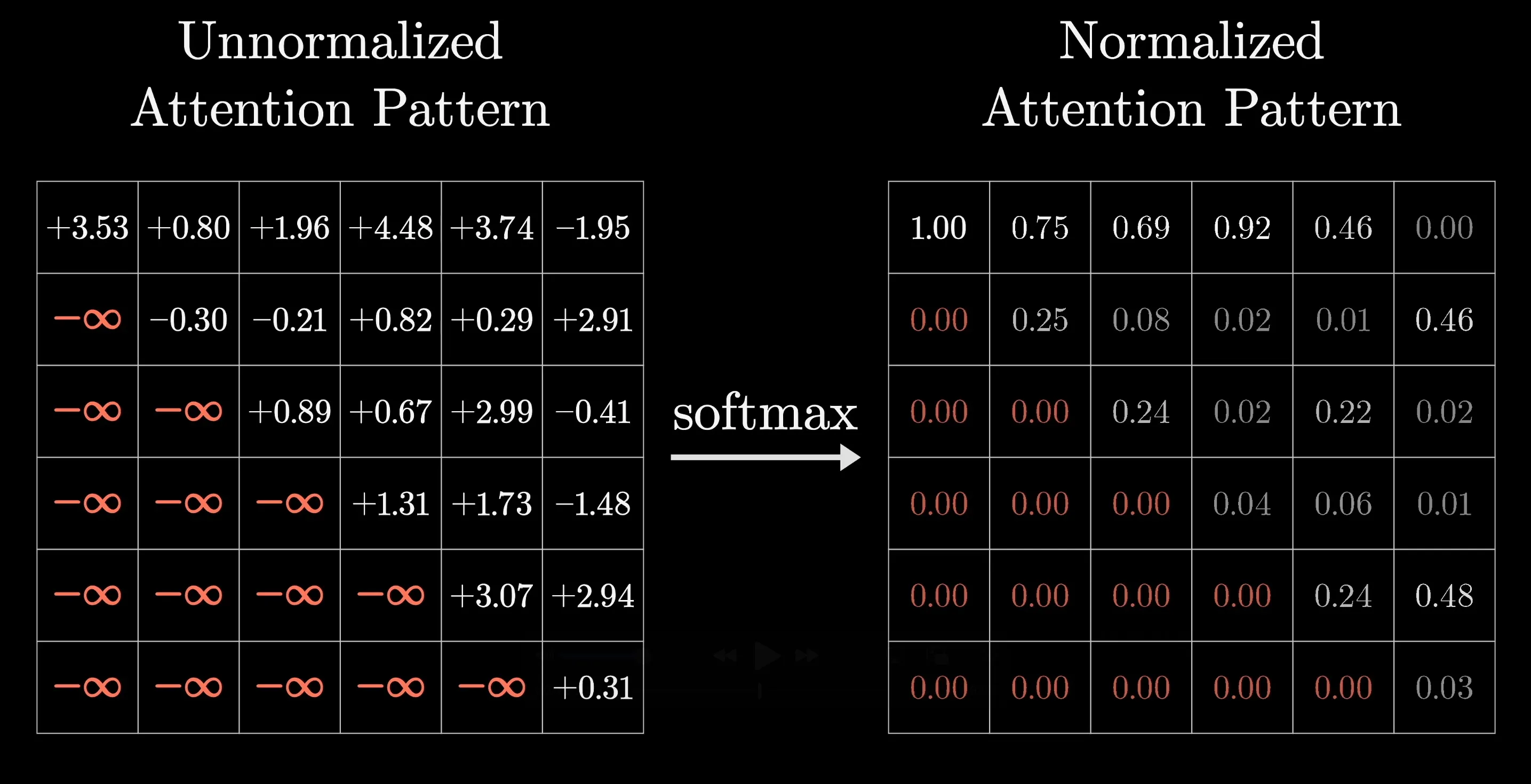Figure 14: Masking sets the upper-triangular scores in the Attention Pattern to $-\infty$ prior to softmax to prevent attention from flowing backwards from future tokens.

Another fact is that this reflecting how the size of this attention is equal to context size

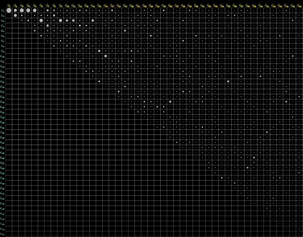Figure 15: The dimensions of the Attention Pattern grid correspond directly to the model’s context size.

This is why the context size could act as a significant limitation for large language models and why scaling up is nontrivial. But of course, motivated by the larger context window, in recent years, some variations have been released but for now let’s start at the basics.

Deep Dive: Value Vectors ($V$)

Once you have this attention pattern describing the relationship between the tokens, the next step is to actually update those embeddings.

The most straightforward way is like the other 2 steps, which uses a third learned matrix called the Value Matrix ($W_V$). The result of this is what we call a Value vector ($\vec{V}$), which represents the information to add to other words to update their meanings.

$\vec{V}_j = W_V \vec{E}_j$

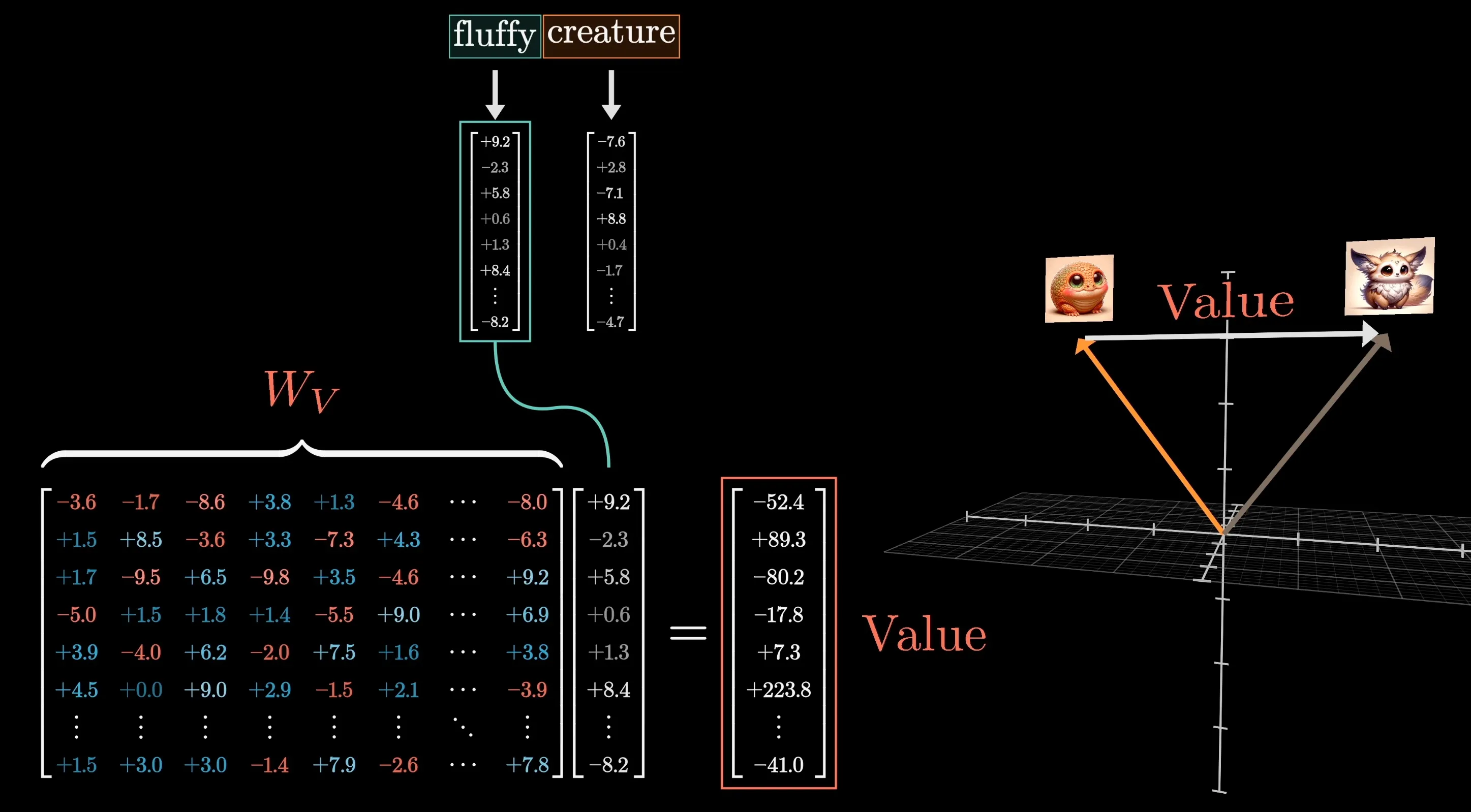Figure 16: Multiplying the embedding of “fluffy” by $W_V$ creates a Value vector. When added to “creature”, the updated embedding now encodes the combined meaning of “fluffy creature”.

As in the image, creature is somehow updated by the word fluffy, the new vector embedding encodes the meaning of fluffy creature. Seems familiar now? This is the main idea inside Token Ingestion.

This Value matrix is multiplied with every one of those embeddings to produce a sequence of Value vectors in parallel:

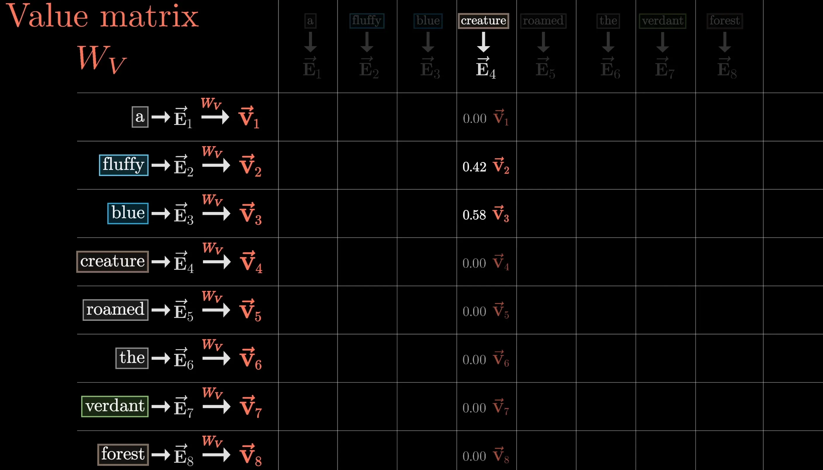Figure 17: Each token embedding $\vec{E}_i$ is projected by $W_V$ into its corresponding Value vector $\vec{V}_i$ in parallel.

Updating the Token Embeddings ($\Delta \vec{E}$)

Now, we combine the Attention Pattern weights with the Value vectors.

For each token, we compute a weighted sum of all Value vectors based on their attention weights, producing a change vector $\Delta \vec{E}$:

$\Delta \vec{E}_i = \sum_j \text{Attention}(i, j) \cdot \vec{V}_j$

In matrix notation, this is the final $V$ term in the Attention Formula:

$\text{Attention}(Q, K, V) = \text{softmax}\left(\frac{Q K^T}{\sqrt{d_k}}\right) V$

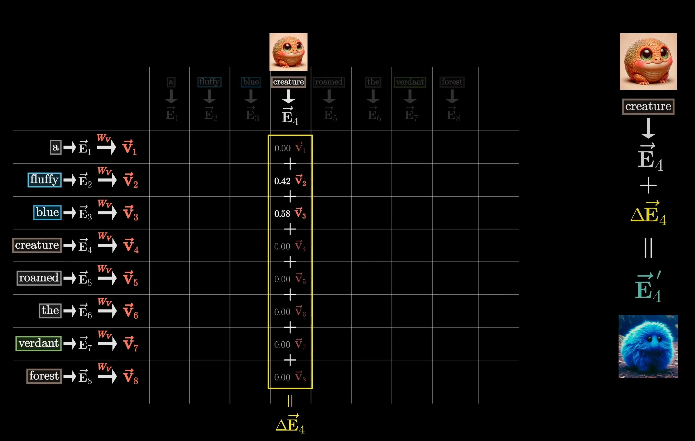Figure 18: The weighted sum of Value vectors produces $\Delta \vec{E}$, which is added to the original embedding $\vec{E}$ to yield the enriched contextual representation $\vec{E}'$.

Finally, this change vector is added back to the original token embedding:

$\vec{E}_i' = \vec{E}_i + \Delta \vec{E}_i$

Now, each token’s vector representation is no longer static — it has absorbed all the relevant context from the surrounding sequence!

Counting Parameters (GPT-3 Example)

Let’s take a moment to count up the parameters introduced by a single attention head using concrete numbers from GPT-3:

• Embedding Dimension ($d_{\text{model}}$): $12,288$
• Key-Query Space Dimension ($d_k$): $128$

Key & Query Matrices ($W_K, W_Q$)

Each Query and Key matrix projects the $12,288$-dimensional embedding space down into a $128$-dimensional subspace:

$\text{Parameters per matrix} = 128 \times 12,288 = 1,572,864 \text{ parameters}$

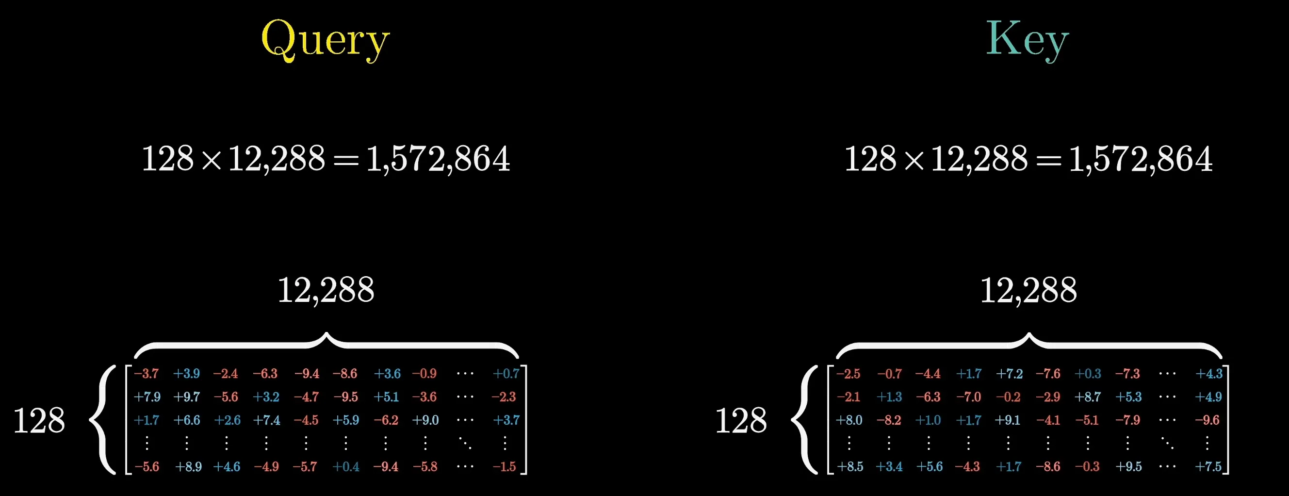Figure 19: In GPT-3, the Query and Key projection matrices have dimensions $128 \times 12,288$, adding ~1.57M parameters each.

Value Matrix ($W_V$) & Parameter Efficiency

If the Value matrix mapped directly from the embedding space back into the embedding space, it would be a massive square matrix ($12,288 \times 12,288$), requiring $150,994,944$ parameters — nearly 100× more than the Query and Key matrices!

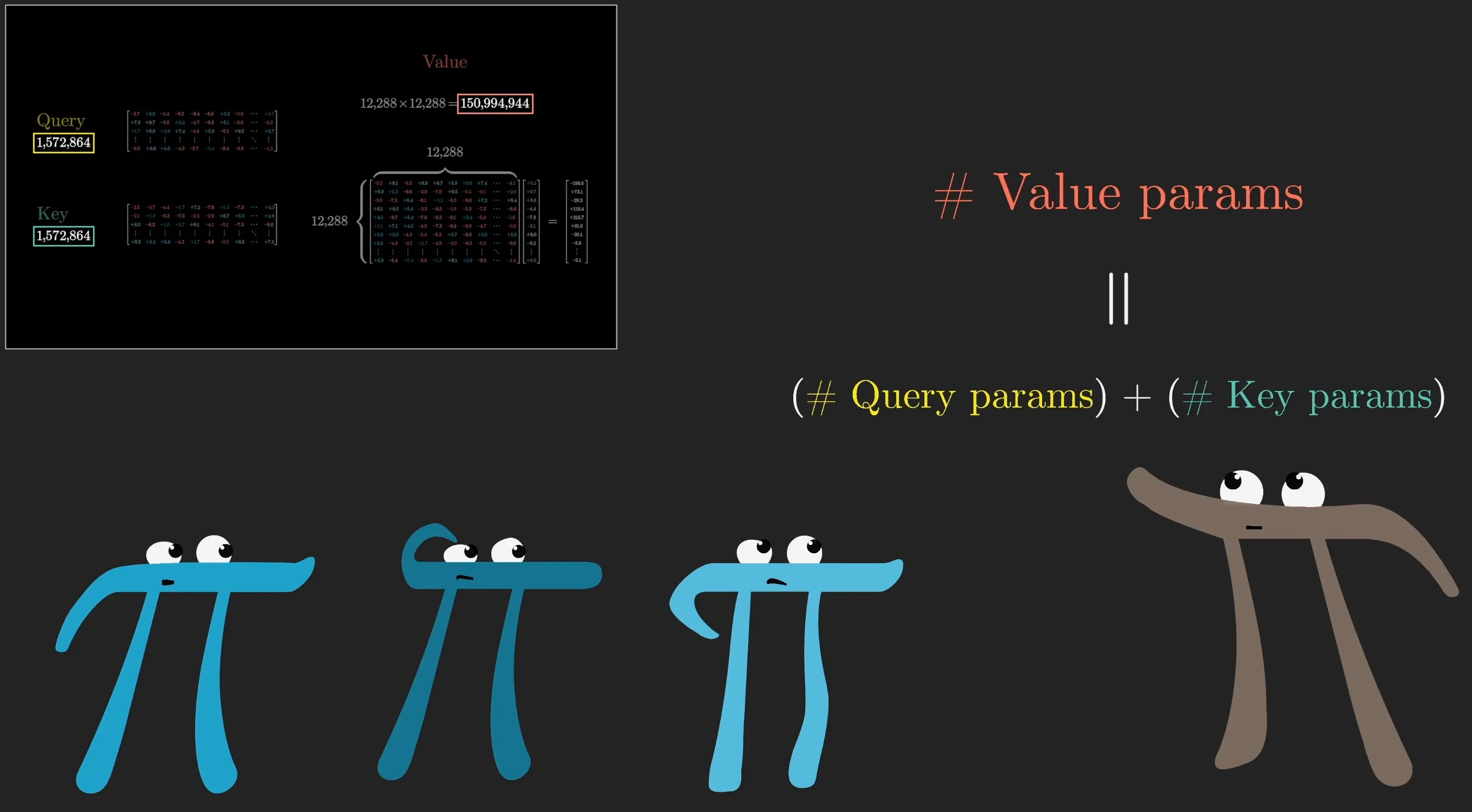Figure 20: Reducing the parameter to match the Query and Key matrices.

In practice, Transformers keep this computationally efficient:

• The Value projection matrix also projects down into a smaller subspace ($d_v = 128$), allocating the exact same parameter budget ($1,572,864$ parameters) as $W_Q$ and $W_K$.
• An output projection matrix then maps the aggregated result back into the full $12,288$-dimensional embedding space.

In Linear Algebra terms, what we’re doing is mapping the bigger space to a smaller space which is called low-rank transformation.

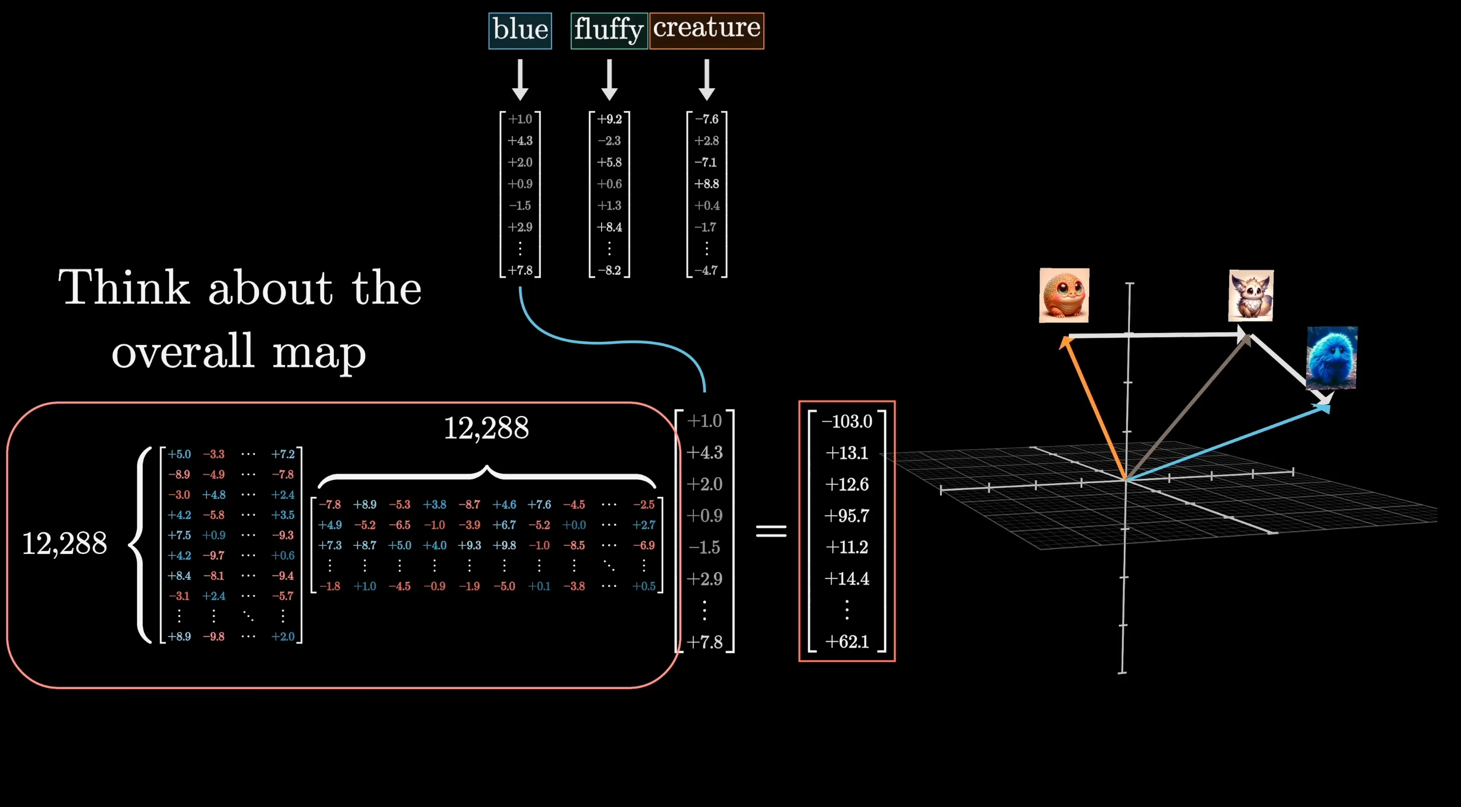Figure 21: Low-rank transformation factors a large $12,288 \times 12,288$ mapping into two smaller matrices ($128 \times 12,288$ and $12,288 \times 128$), vastly reducing parameters.

Going back to the parameter count of GPT-3, all four of these matrices have the same size, and by adding those up we get about 6.3 million parameters for one attention head.

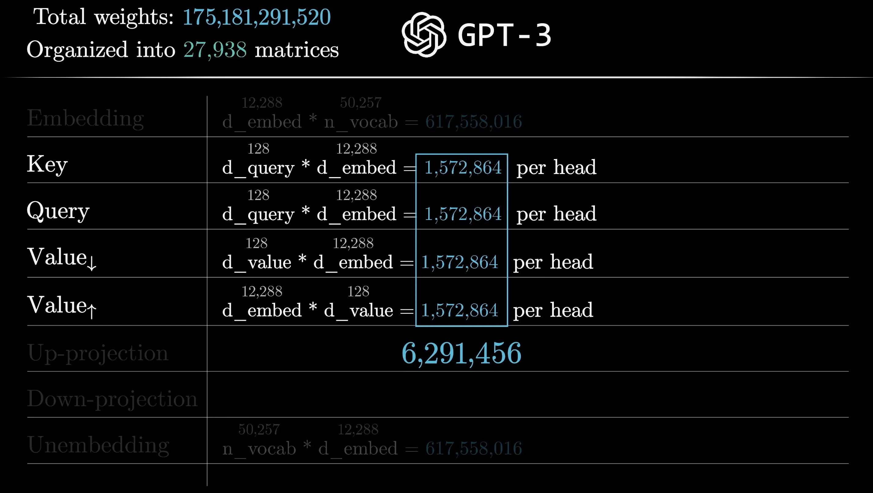Figure 22: All four matrices ($W_Q, W_K, W_V, W_O$) in one GPT-3 attention head contribute $4 \times 1,572,864 \approx 6.3\text{M}$ parameters in total.

Cross-Attention

As a quick note, all what we are talked about so far is called self-attention, which is different from a variation called cross-attention.

A cross-attention head is involved in models that process two distinct types of data, like text in one language and text in another language that’s part of an ongoing generation of a translation.

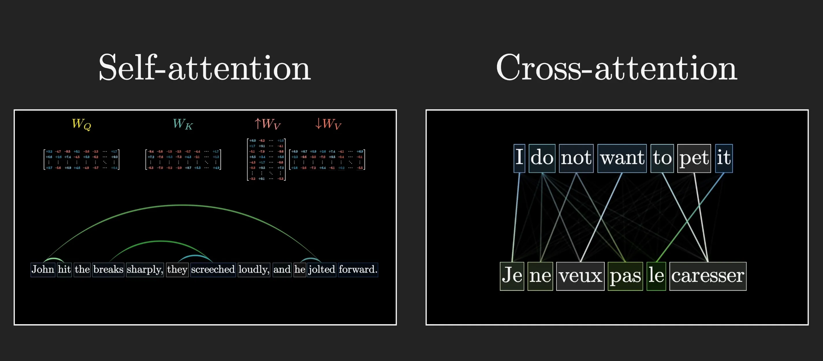Figure 23: Cross-attention connects two different data streams (e.g., source language and target language translation).

A cross-attention head looks almost identical to a self-attention head, with the only difference being that the key and query maps act on different data sets.

In a model doing translation, for example, the keys might come from one language, while the queries come from another, and the attention pattern could tell relevance of words from one language correspond to which words in another.

And notice that in this setting there would typically be no masking, since there’s not really any notion of later tokens affecting earlier ones.

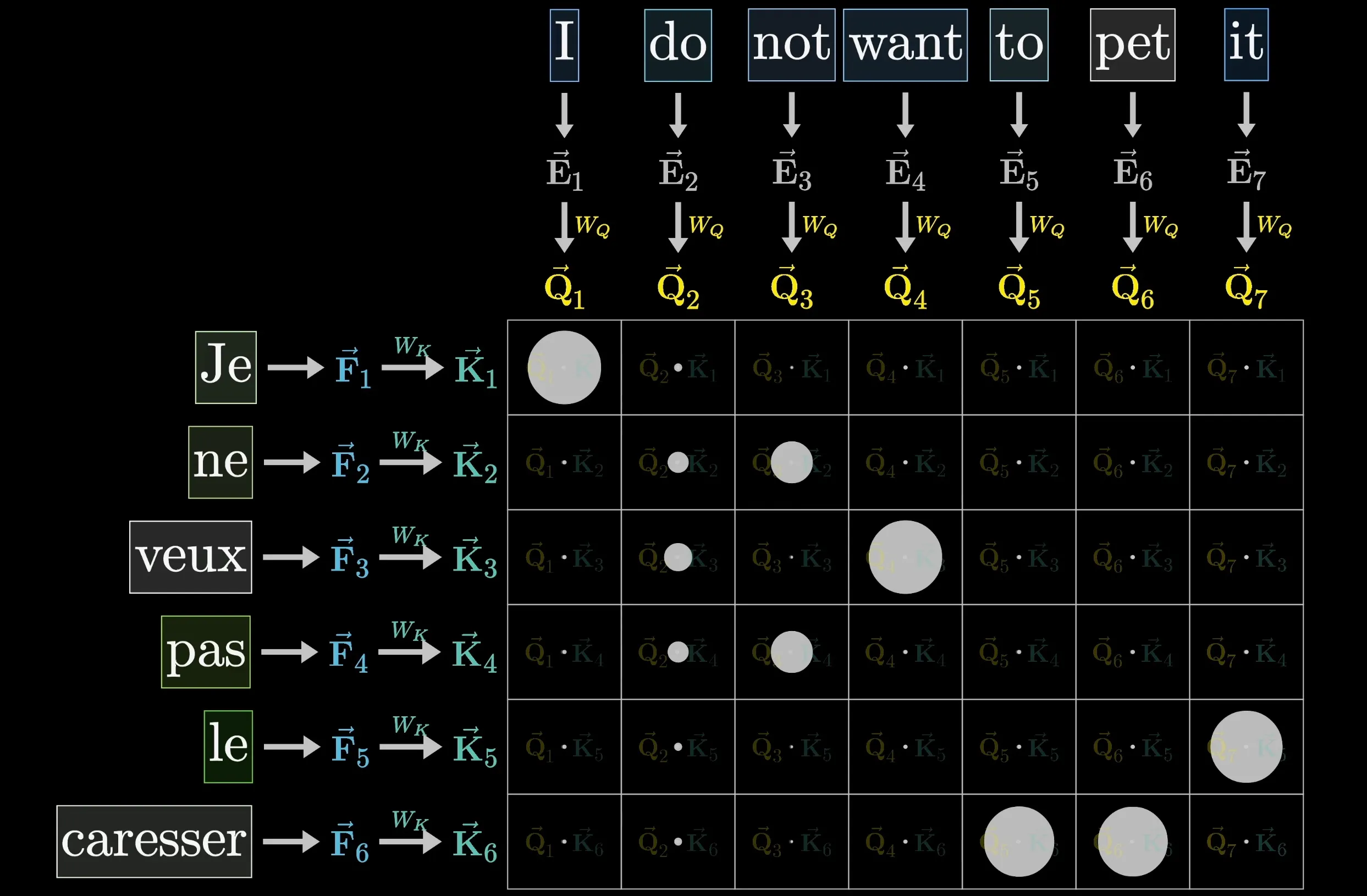Figure 24: In cross-attention, Queries come from the target sequence while Keys and Values come from the source sequence, producing an unmasked alignment grid across data streams.

Multi-Headed Attention

• All the information we have covered so far is contained in a single head of attention.
• In modern LLMs, a full attention block consists of multiple heads running in parallel, which is called Multi-Headed Attention, where operations run simultaneously with distinct Key, Query, and Value weight matrices.

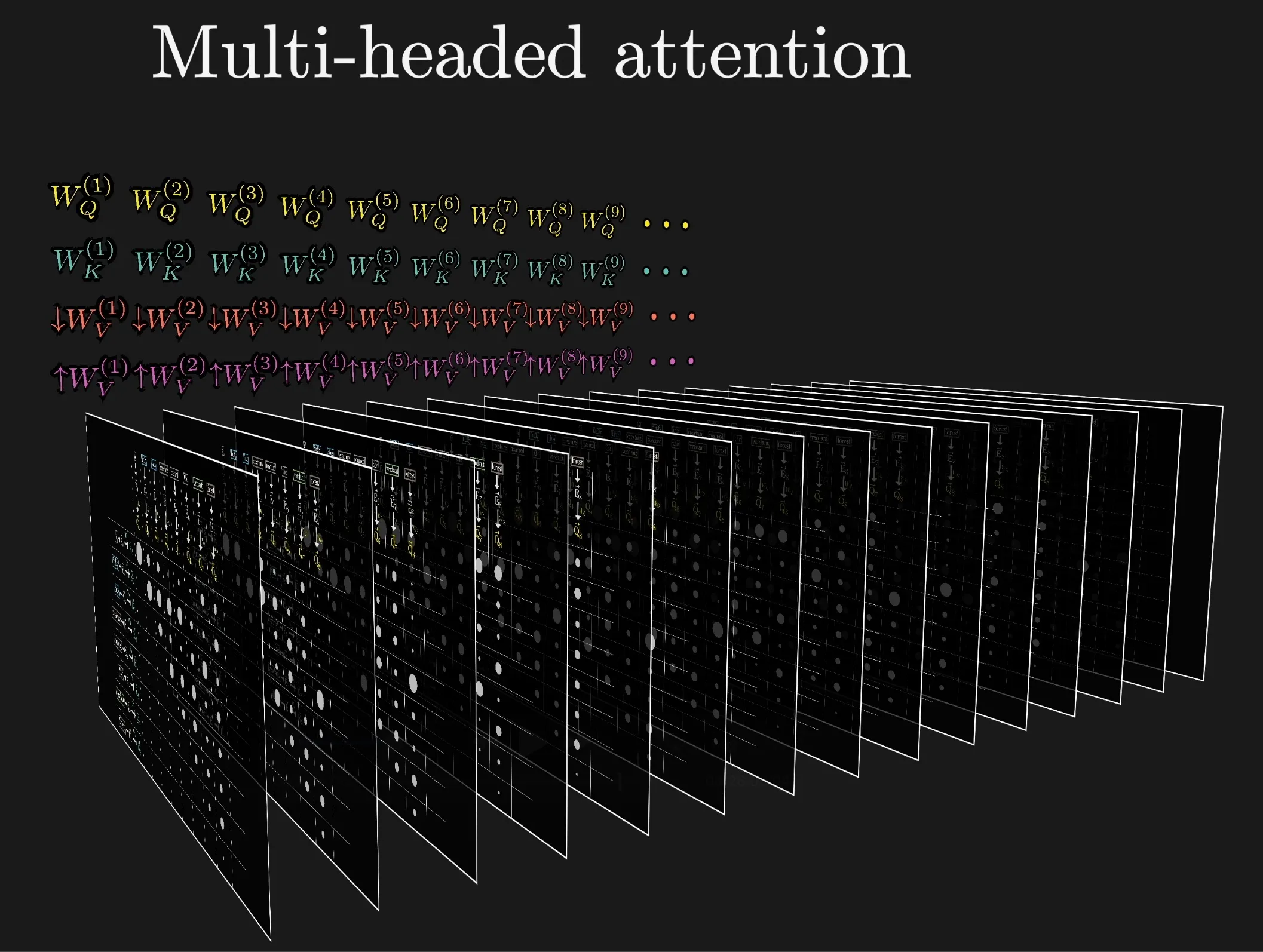Figure 25: Multi-Headed Attention runs many attention heads simultaneously (e.g., 96 heads in GPT-3), allowing the model to capture multiple distinct relationships at once.

Each head has its own independent Query, Key, and Value matrices ($W_Q^{(h)}, W_K^{(h)}, W_V^{(h)}$) and computes its attention pattern in parallel:

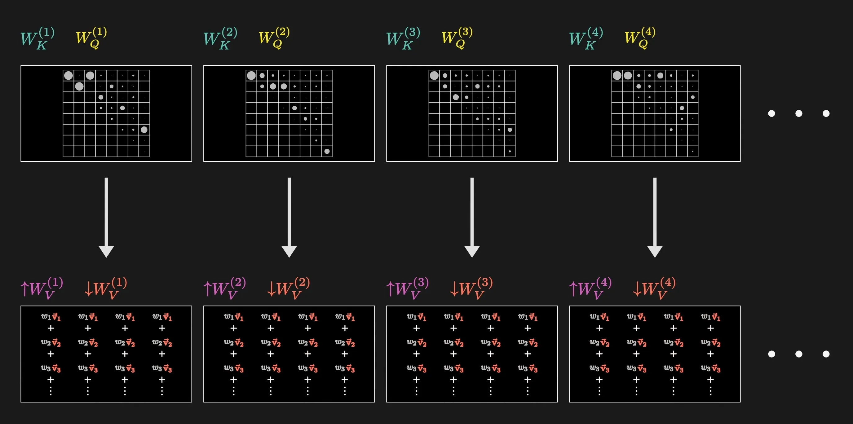Figure 26: Each attention head performs its own QKV projections and attention pattern calculations in parallel.

Aggregating Multi-Head Updates

Each attention head produces its own delta vector ($\Delta \vec{E}^{(h)}$) representing the specialized context it gathered:

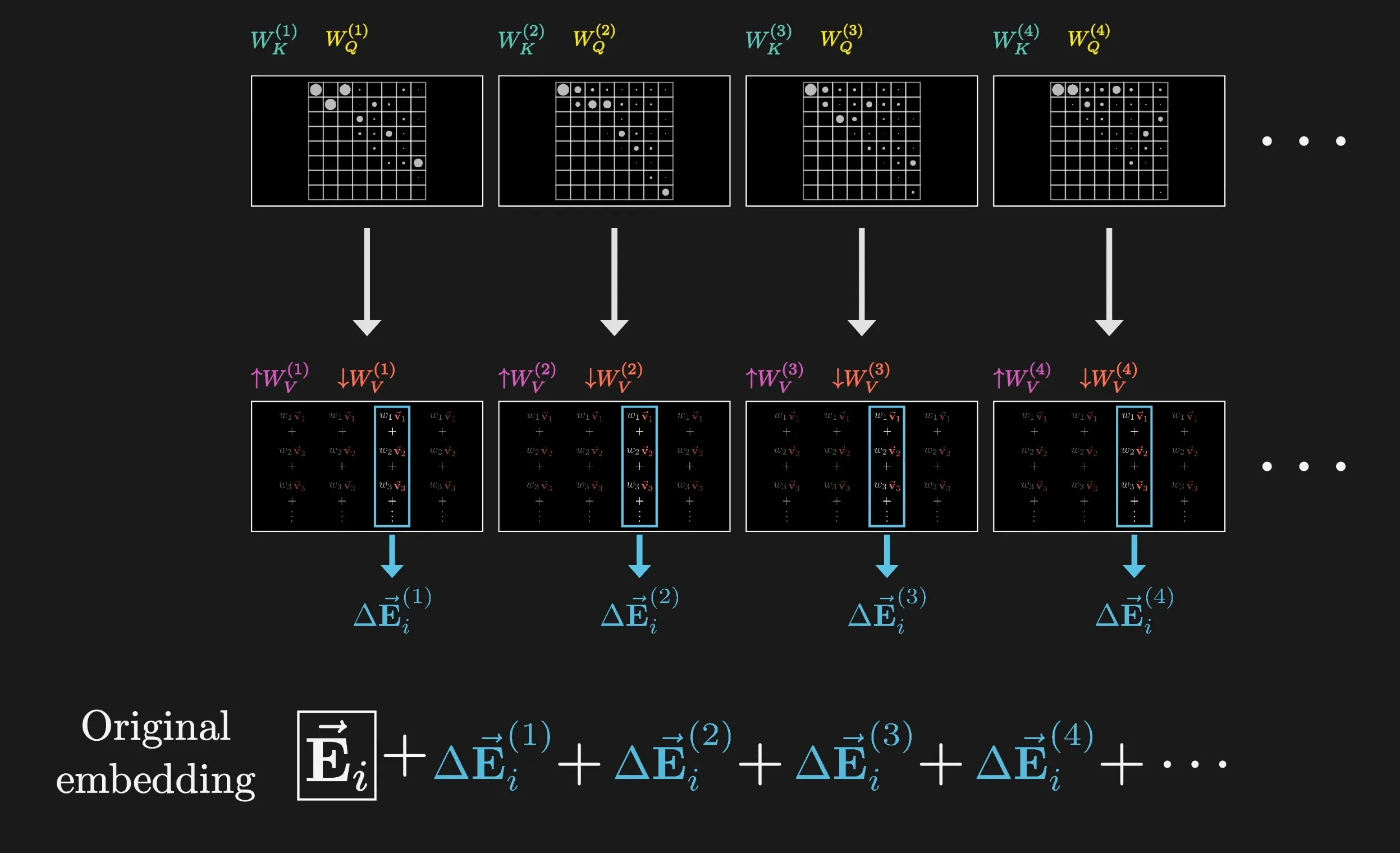Figure 27: Every attention head computes a separate change vector ($\Delta \vec{E}^{(h)}$) corresponding to its specialized focus.

Finally, the updates from all heads are combined and added back into the original embedding:

$\vec{E}' = \vec{E} + \Delta \vec{E}_{\text{multi-head}}$

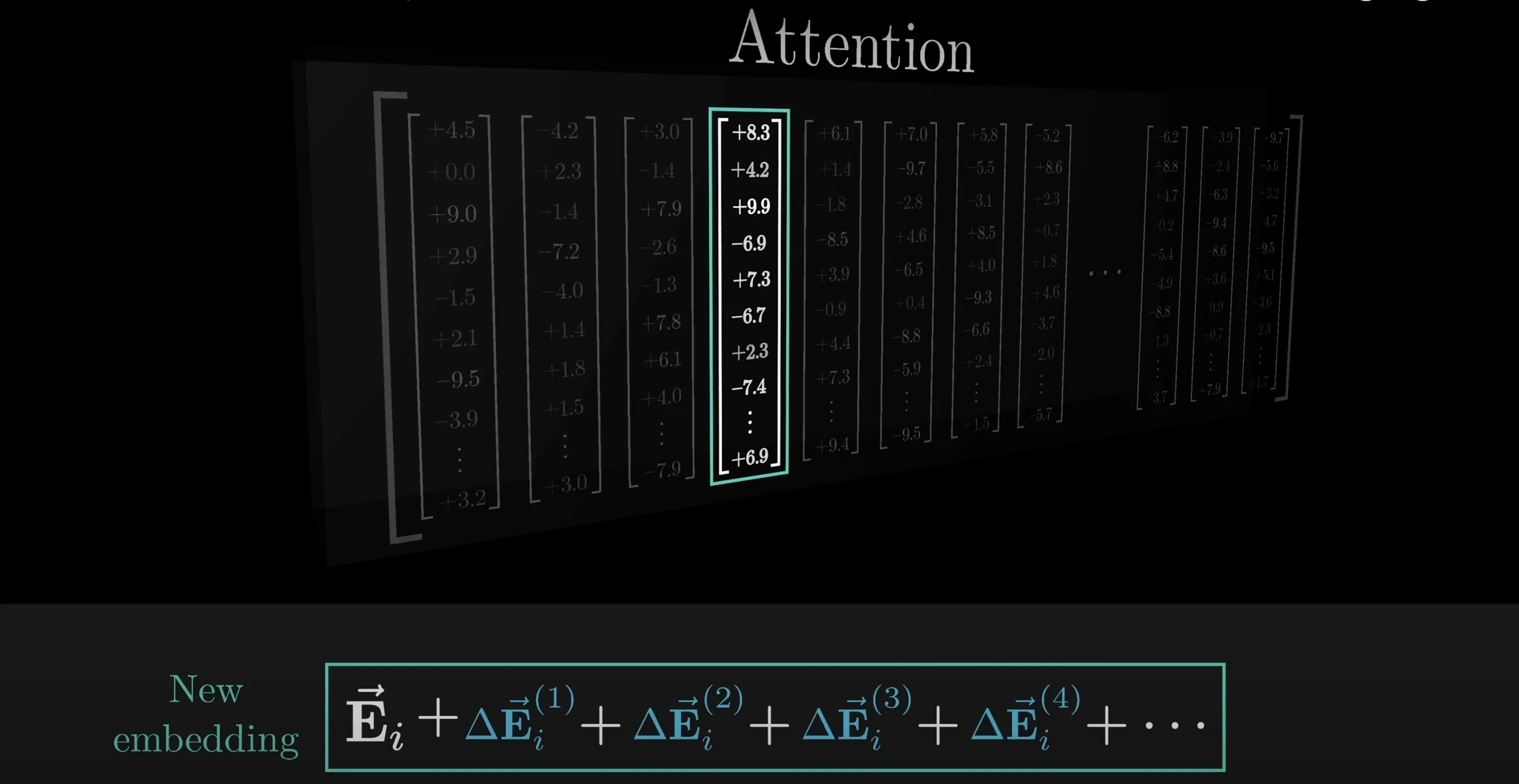Figure 28: The outputs of all attention heads are aggregated and added to the original embedding, producing a rich, multi-faceted contextual representation.

Summary

In modern Transformer architectures:

1. Queries ($Q$) broadcast what information a token is looking for.
2. Keys ($K$) advertise what information a token contains.
3. Attention Pattern calculates how relevant each token is to every other token using $\text{softmax}(Q K^T / \sqrt{d_k})$.
4. Values ($V$) provide the actual content to transfer, computing a delta vector $\Delta \vec{E}$ that updates each token’s embedding with context.
5. Cross-Attention: Queries and Keys/Values originate from two distinct sequences (e.g. translation or multimodal tasks) without causal masking.
6. Multi-Headed Attention: Runs dozens of independent attention heads in parallel to capture diverse linguistic and contextual relationships simultaneously.
7. Low-rank transformation: Reduce matrix dimensions to save parameters while preserving expressivity.