Linear Regression from Scratch with PyTorch

Linear Regression is the simplest and most important starting point in Machine Learning. In this post, we apply it to a well-known benchmark: the Kaggle House Prices competition, building the whole pipeline from scratch with PyTorch.

Table of contents

1. Problem: House Price Prediction

Given house features (like area, neighborhood, year built), our goal is to predict the final sale price:

• Input ($\mathbf{x}$): House features (both numbers and text categories).
• Target ($y$): SalePrice in USD.
• Goal: Find a model $f(\mathbf{x}) \approx y$.

2. Math Formulation

Linear Regression assumes the target is a linear combination of input features:

Where:

• $\mathbf{w}$ is the weights vector (slope per feature).
• $b$ is the bias scalar (baseline intercept).
• $\hat{y}$ is the predicted price.

For a batch of $n$ houses $\mathbf{X} \in \mathbb{R}^{n \times d}$:

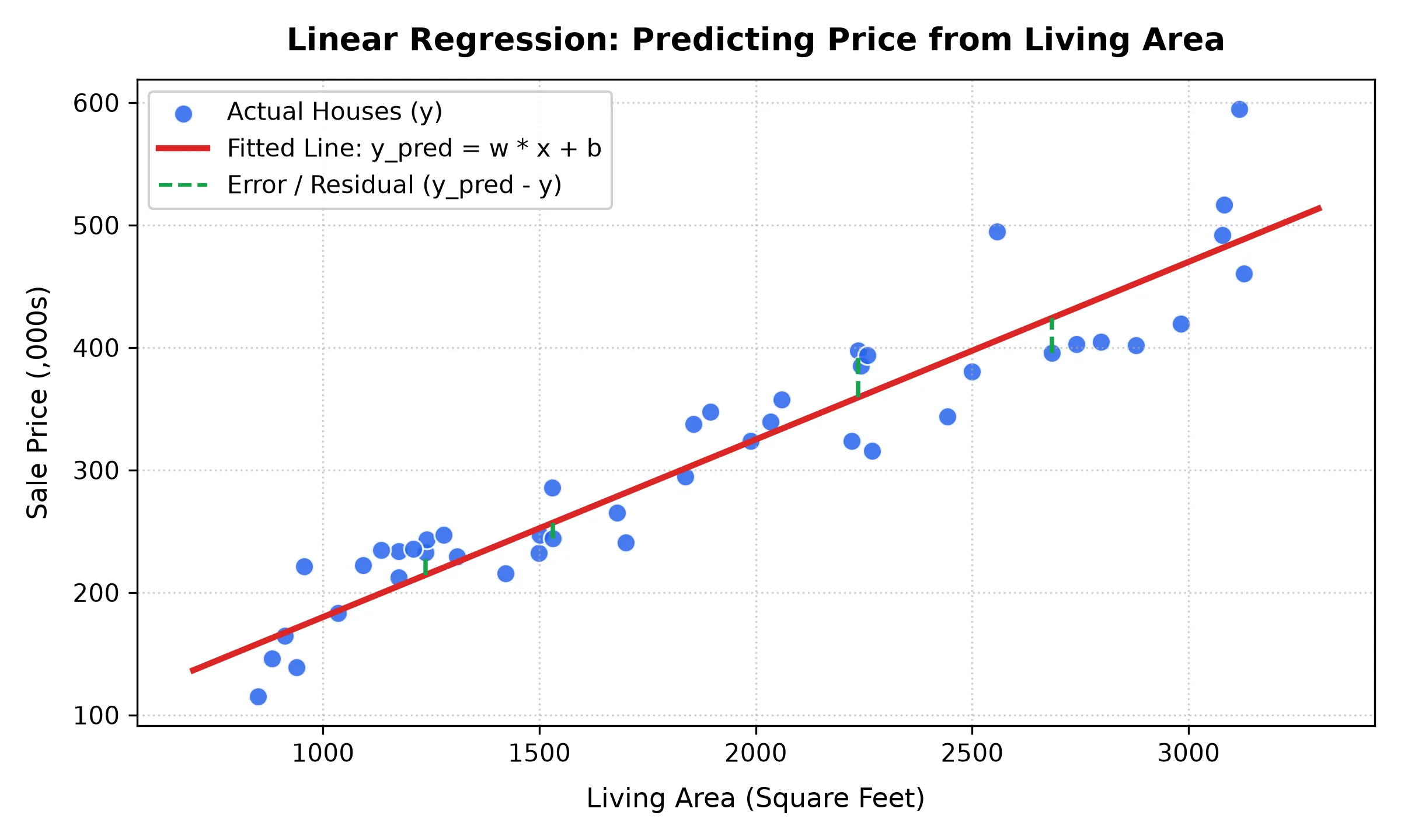Figure 1: Fitting a linear model to house area vs. sale price. Green dashed lines show the residual errors $(\hat{y} - y)$ that the loss function minimizes.

3. Loss & Optimization

MSE Loss

We measure error using Mean Squared Error:

Mini-Batch Stochastic Gradient Descent

Instead of computing the gradient over the whole dataset (too slow) or a single sample (too noisy), we sample a small random mini-batch $\mathcal{B}_t$ of size $|\mathcal{B}|$ and update parameters using its average gradient:

Where:

• $|\mathcal{B}|$ is the batch size (e.g., 64).
• $\eta$ is the learning rate.
• $\left( \mathbf{w}^\top \mathbf{x}^{(i)} + b - y^{(i)} \right)$ is the prediction error $(\hat{y}^{(i)} - y^{(i)})$.

4. Data Preprocessing

Raw data has missing values, text columns, and large numbers that need cleaning first:

1. Different Scales & Missing Numbers

• Problem: Features have very different scales (LotArea is in thousands, while OverallQual is 1 to 10). Large numbers will dominate gradient updates. Also, missing numbers (NaN) break matrix math.
• Solution: Use Z-score normalization so all numbers have mean $0$ and variance $1$: $$x' = \frac{x - \mu}{\sigma}$$ Then replace missing values (NaN) with $0$ (which is the mean value).

2. Text (Categorical) Features

• Problem: Models only understand numbers, not text labels like "CollgCr" or "Crawfor".
• Solution: Use One-Hot Encoding to turn text categories into binary $0/1$ columns. Missing categories become their own dummy column.

3. Skewed Price Distribution

• Problem: House prices are unevenly distributed (a few luxury houses are huge outliers). Also, predicting $120k for a $100k house and $1,020k for a $1,000,000 house both have the same absolute error ($20k), but very different relative errors (20% vs 2%). Standard MSE penalizes them equally.
• Solution: Take the natural log of prices:

Why does this measure relative error? (Math intuition)

From basic calculus and logarithm properties:

(using the Taylor approximation $\log(1 + \delta) \approx \delta$ for small errors $\delta$).

Thus, minimizing MSE in log-space:

directly minimizes the relative percentage error (Kaggle’s official RMSLE metric), treating a 10% error on a cheap house with the exact same weight as a 10% error on a luxury mansion. At test time, we convert predictions back using $\exp(\hat{y}_{\text{log}})$.

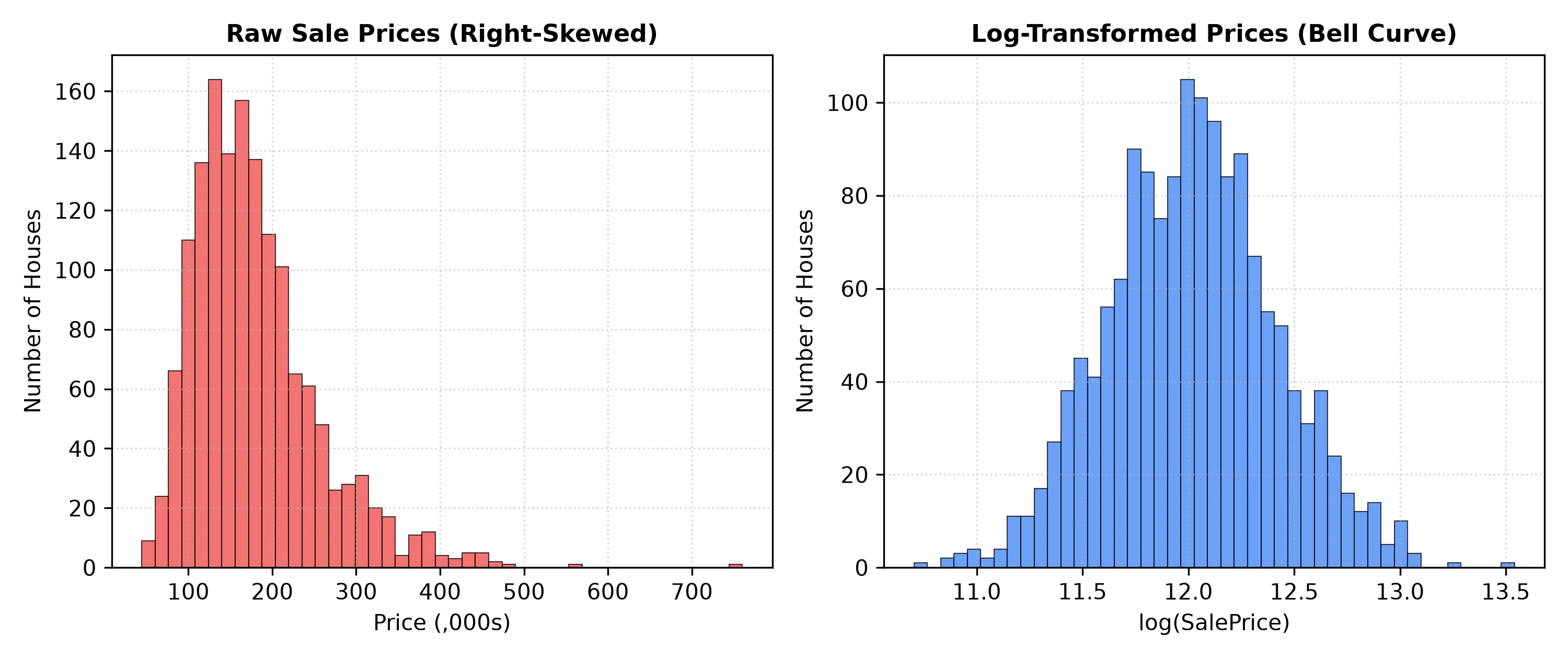Figure 2: Raw sale prices are heavily skewed to the right (left). Applying $\log(\text{SalePrice})$ produces a symmetric bell-shaped normal distribution (right), stabilizing gradient updates.

5. Implementation from Scratch

import pandas as pd
import torch
import random

class DataModule:
    def __init__(self, train_path: str, test_path: str, batch_size: int = 64, train_ratio: float = 0.8):
        self.train_path = train_path
        self.test_path = test_path
        self.batch_size = batch_size
        self.train_ratio = train_ratio

        self.X_train = None
        self.y_train = None
        self.X_val = None
        self.y_val = None
        self.X_test = None
        self.X_test_id = None

    def preprocess(self):
        raw_train_data = pd.read_csv(self.train_path)
        raw_test_data = pd.read_csv(self.test_path)
        self.X_test_id = raw_test_data["Id"]

        # 1. Feature Alignment
        features = pd.concat(
            [
                raw_train_data.drop(columns=["Id", "SalePrice"]),
                raw_test_data.drop(columns=["Id"]),
            ],
            ignore_index=True,
        )

        # 2. Standardization & Imputation
        numerical_cols = features.select_dtypes(include=["number"]).columns
        features[numerical_cols] = features[numerical_cols].apply(
            lambda x: (x - x.mean()) / x.std()
        )
        features[numerical_cols] = features[numerical_cols].fillna(0)

        # 3. One-Hot Encoding
        features = pd.get_dummies(features, dummy_na=True, dtype=float)

        # 4. Partition and Convert to Tensors
        num_train_data = raw_train_data.shape[0]
        num_test_data = raw_test_data.shape[0]
        train_size = int(num_train_data * self.train_ratio)

        all_X_train = torch.tensor(
            features[:num_train_data].to_numpy(), dtype=torch.float32
        )
        all_y_train = torch.log(
            torch.tensor(raw_train_data["SalePrice"].to_numpy(), dtype=torch.float32)
        ).reshape(-1, 1)

        self.X_train = all_X_train[:train_size]
        self.y_train = all_y_train[:train_size]
        self.X_val = all_X_train[train_size:]
        self.y_val = all_y_train[train_size:]

        self.X_test = torch.tensor(
            features[num_train_data:].to_numpy(), dtype=torch.float32
        )

    def get_batch(self, train: bool = True):
        X = self.X_train if train else self.X_val
        y = self.y_train if train else self.y_val
        assert X is not None and y is not None, "DataModule must be preprocessed first."

        data_size = X.shape[0]
        indices = list(range(data_size))
        if train:
            random.shuffle(indices)

        for i in range(0, data_size, self.batch_size):
            batch_idx = indices[i : min(data_size, i + self.batch_size)]
            yield (X[batch_idx], y[batch_idx])

4. Model Architecture & Custom Optimizer

Model Class

class LinearRegression:
    def __init__(self, num_features: int, learning_rate: float, sigma: float = 0.01):
        self.learning_rate = learning_rate
        self.W = torch.normal(0, sigma, (num_features, 1), requires_grad=True)
        self.b = torch.zeros(1, requires_grad=True)

    def forward(self, X: torch.Tensor) -> torch.Tensor:
        return torch.matmul(X, self.W) + self.b

    def loss(self, y_hat: torch.Tensor, y: torch.Tensor) -> torch.Tensor:
        return (((y_hat.reshape(y.shape) - y) ** 2) / 2).mean()

    def training_step(self, batch):
        X, y = batch[0], batch[1]
        return self.loss(self.forward(X), y)

    def validation_step(self, batch):
        X, y = batch[0], batch[1]
        return self.loss(self.forward(X), y)

    def configure_optimizer(self):
        return Stochastic_Gradient_Descent([self.W, self.b], self.learning_rate)

Custom SGD Optimizer

class Stochastic_Gradient_Descent:
    def __init__(self, params, learning_rate: float):
        self.params = params
        self.learning_rate = learning_rate

    def step(self):
        with torch.no_grad():
            for param in self.params:
                if param.grad is not None:
                    param -= self.learning_rate * param.grad

    def grad_zero(self):
        for param in self.params:
            if param.grad is not None:
                param.grad.zero_()

5. Training Loop & Convergence Analysis

The training coordinator manages the forward-backward cycle across mini-batches while detaching scalar metrics via .item() to prevent graph accumulation:

class Trainer:
    def __init__(self, num_epochs: int):
        self.num_epochs = num_epochs
        self.train_loss_history = []
        self.val_loss_history = []

    def fit(self, model: LinearRegression, data_module: DataModule):
        optim = model.configure_optimizer()
        for epoch in range(self.num_epochs):
            total_train_loss = 0.0
            num_train_batch = 0
            for batch in data_module.get_batch(train=True):
                train_loss = model.training_step(batch)
                total_train_loss += train_loss.item()
                num_train_batch += 1

                optim.grad_zero()
                train_loss.backward()
                optim.step()

            total_val_loss = 0.0
            num_val_batch = 0
            with torch.no_grad():
                for batch in data_module.get_batch(train=False):
                    val_loss = model.validation_step(batch)
                    total_val_loss += val_loss.item()
                    num_val_batch += 1

            self.train_loss_history.append(total_train_loss / max(num_train_batch, 1))
            self.val_loss_history.append(total_val_loss / max(num_val_batch, 1))

Visualizing Loss Progression

import matplotlib.pyplot as plt

class LossPlotter:
    def __init__(self, train_loss_history, val_loss_history):
        self.train_loss_history = train_loss_history
        self.val_loss_history = val_loss_history

    def plot(self, save_path=None):
        epochs = range(1, len(self.train_loss_history) + 1)
        plt.figure(figsize=(7, 4))
        plt.plot(epochs, self.train_loss_history, label="Train Loss", color="blue")
        plt.plot(epochs, self.val_loss_history, label="Val Loss", color="red", linestyle="--")
        plt.xlabel("Epoch")
        plt.ylabel("MSE Loss")
        plt.title("Training and Validation Loss")
        plt.legend()
        plt.grid(True)
        if save_path:
            plt.savefig(save_path)
        plt.close()

Main Pipeline Execution

if __name__ == "__main__":
    current_dir = os.path.dirname(os.path.abspath(__file__))
    train_path = os.path.join(
        current_dir, "house-prices-advanced-regression-techniques", "train.csv"
    )
    test_path = os.path.join(
        current_dir, "house-prices-advanced-regression-techniques", "test.csv"
    )

    # 1. Preprocess Data
    data_module = DataModule(
        train_path=train_path,
        test_path=test_path,
        batch_size=64,
        train_ratio=0.8,
    )
    data_module.preprocess()

    # 2. Initialize Model & Trainer
    num_features = data_module.X_train.shape[1]
    model = LinearRegression(
        num_features=num_features,
        learning_rate=0.03,
        sigma=0.01,
    )
    trainer = Trainer(num_epochs=100)

    # 3. Fit Model
    trainer.fit(model, data_module)

    # 4. Plot Convergence
    plotter = LossPlotter(trainer.train_loss_history, trainer.val_loss_history)
    plotter.plot(save_path=os.path.join(current_dir, "loss_plot.png"))

    # 5. Predict on Test Set & Save Submission
    with torch.no_grad():
        y_test_pred = model.forward(data_module.X_test)
        real_house_prices = torch.exp(y_test_pred).detach().reshape(-1).numpy()
        submission = pd.DataFrame(
            {"Id": data_module.X_test_id, "SalePrice": real_house_prices}
        )
        submission.to_csv(os.path.join(current_dir, "submission.csv"), index=False)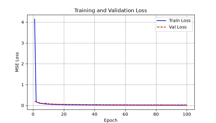

Figure 3: Training MSE (blue) and Validation MSE (red dashed) converging smoothly across epochs without diverging.

6. Kaggle Submission & Verification

After training the model on the preprocessed dataset, we generate predictions for the test set test.csv by exponentiating the model output: $\hat{y} = \exp(\hat{y}_{\text{log}})$.

Submitting our predictions to the House Prices: Advanced Regression Techniques leaderboard confirms the performance of our from-scratch model:

Figure 4: Our final submission score on Kaggle, verifying the effectiveness of clean data preprocessing combined with mini-batch SGD.

By decoupling data processing, parameter optimization, and visual evaluation, we obtain a transparent and robust pipeline that is mathematically faithful to the core principles of deep learning.