In Machine Learning, Regression is the tool we use to answer “How much?” or “How many?” (such as predicting a house price). Classification, on the other hand, answers “Which category?”:
- Does this email belong in the spam folder?
- Is this image a cat, a dog, or a chicken?
Even though the question changes, the core training pipeline stays the same: load data, pass it through the model, calculate loss, compute gradients, and update weights. What changes are how we represent labels, the shape of the output layer, and the loss function.

Table of contents
Open Table of contents
1. Types of Classification
When classifying data, we usually distinguish between:
- Hard Assignment: Picking one exact class label right away (e.g., “This is definitely a dog”).
- Soft Assignment: Predicting the probability of every possible class (e.g., 85% dog, 10% cat, 5% chicken). In practice, models output soft probabilities first, and we pick the highest one to make a hard decision.
- Multi-Label Classification: When a single item can belong to multiple categories at once (for example, a news article that is about business, technology, and space flight at the same time).
2. Representing Labels: Why One-Hot Encoding?
How should we turn words like {dog, cat, chicken} into numbers for our model?
The Trap of Integer Encoding
A natural first thought is to assign each class a number:
When integer labels work: If your categories have a natural order (Ordinal Data), like age groups {baby = 1, child = 2, adult = 3}, integers make sense because reflects real-world order.
However, for normal categories like {dog, cat, chicken}, there is no natural order. Using tricks the math into assuming two false rules:
- “Chicken” () is greater than “Dog” ().
- The distance between “Dog” () and “Cat” () is , while the distance between “Dog” () and “Chicken” () is — implying a dog is mathematically closer to a cat than a chicken!
The Solution: One-Hot Encoding
To remove this fake ordering, we use One-Hot Encoding. We create a vector with one slot per class: the true class gets a , and all other slots get .
For 3 classes {cat, chicken, dog}, our target label becomes a 3-element vector:
Every class is now treated equally at the exact same distance from one another.
Visualizing the Fashion-MNIST Dataset
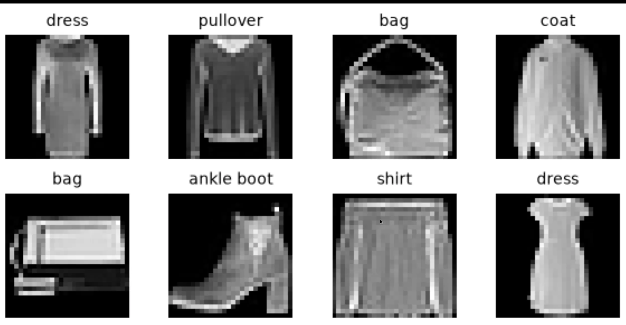
Before building our model, let’s inspect sample images from the Fashion-MNIST dataset along with their ground-truth labels:
Implementing One-Hot Encoding in PyTorch
Here is how we can implement One-Hot Encoding from scratch for our 10 Fashion-MNIST clothing categories:
import torch

labels = [
    "t-shirt", "trouser", "pullover", "dress", "coat",
    "sandal", "shirt", "sneaker", "bag", "ankle boot"
]

def one_hot_encoding(label, classes_name=labels):
    num_classes = len(classes_name)
    vec = torch.zeros(num_classes, dtype=torch.float32)

    if isinstance(label, str):
        if label not in classes_name:
            raise ValueError(f"Label '{label}' is not valid!")
        idx = classes_name.index(label)
    else:
        idx = int(label)

    vec[idx] = 1.0
    return vec

# Example: convert "shirt" (class 6) to a one-hot vector
enc_vector = one_hot_encoding("shirt")
print(enc_vector)
# Output: tensor([0., 0., 0., 0., 0., 0., 1., 0., 0., 0.])PyTorch Built-in (F.one_hot):
In practice, PyTorch has a built-in helper torch.nn.functional.one_hot that vectorizes this across entire mini-batches:
import torch.nn.functional as F

# For a batch of label indices:
y_batch = torch.tensor([6, 1, 3])  # shirt, trouser, dress
print(F.one_hot(y_batch, num_classes=10))
(Note: When using torch.nn.CrossEntropyLoss, PyTorch accepts raw integer class indices directly without requiring manual one-hot encoding).
3. Linear Model for Classification
In Linear Regression, we only needed a single output node to predict one continuous number:
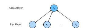
In Classification, to predict probabilities for different classes, our model needs outputs — one score per class.
For example, if we have input features and output classes , we need weights and biases:
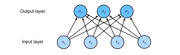
Each output score (called a logit) is calculated as its own linear equation:
In compact matrix form:
Implementing the Linear Model in PyTorch
Here is how we set up the parameters and the forward pass from scratch:
import torch

class ClassificationModel:
    def __init__(
        self,
        num_features: int,
        num_classes: int,
        learning_rate: float = 0.1,
        sigma: float = 0.01,
    ):
        self.num_features = num_features
        self.learning_rate = learning_rate
        # Weights matrix: shape (num_features, num_classes)
        self.W = torch.normal(
            0, sigma, (num_features, num_classes), requires_grad=True
        )
        # Bias vector: shape (num_classes,)
        self.b = torch.zeros(num_classes, requires_grad=True)

    def forward(self, X: torch.Tensor) -> torch.Tensor:
        # Flatten image batches from (batch_size, 1, H, W) to (batch_size, num_features)
        X = X.reshape(-1, self.num_features)
return torch.matmul(X, self.W) + self.bFor Fashion-MNIST, each image is pixels and there are categories. Thus, num_features = 784 and num_classes = 10. The weights matrix will have size , and the bias will have size .
4. The Softmax Function
We cannot use the raw outputs directly as probabilities for two reasons:
- Raw scores can be negative.
- Raw scores do not add up to .
To turn raw logits into valid probabilities, we pass them through the Softmax function in two simple steps:
- Exponentiate (): Forces every score to be strictly positive ().
- Normalize: Divide each positive value by their total sum so they add up to .
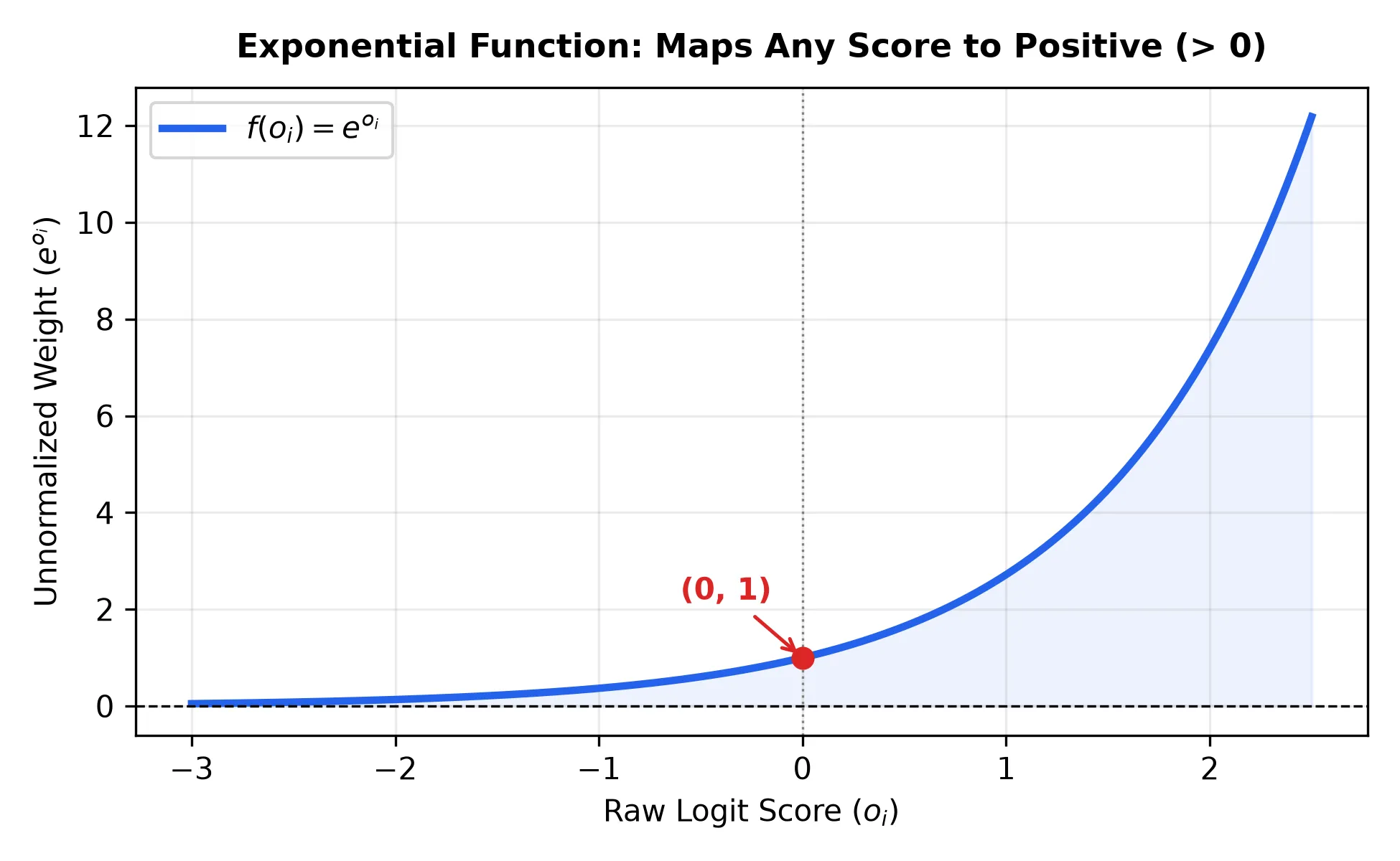
Putting both steps together gives the Softmax equation:
Now is a valid probability distribution where and .
Problem: Overflow and Underflow
Computers store 32-bit floating numbers (float32) within a limited range (approximately to , with a smallest positive limit around ). Because the exponential function explodes rapidly, naive Softmax faces two serious numerical hazards:
- Overflow (): If any score , exceeds the float32 ceiling () and overflows to
inf. - Underflow () and the
NaNDisaster: When a score is large and negative, drops below the computer’s precision limit and gets forced to exact0.0.
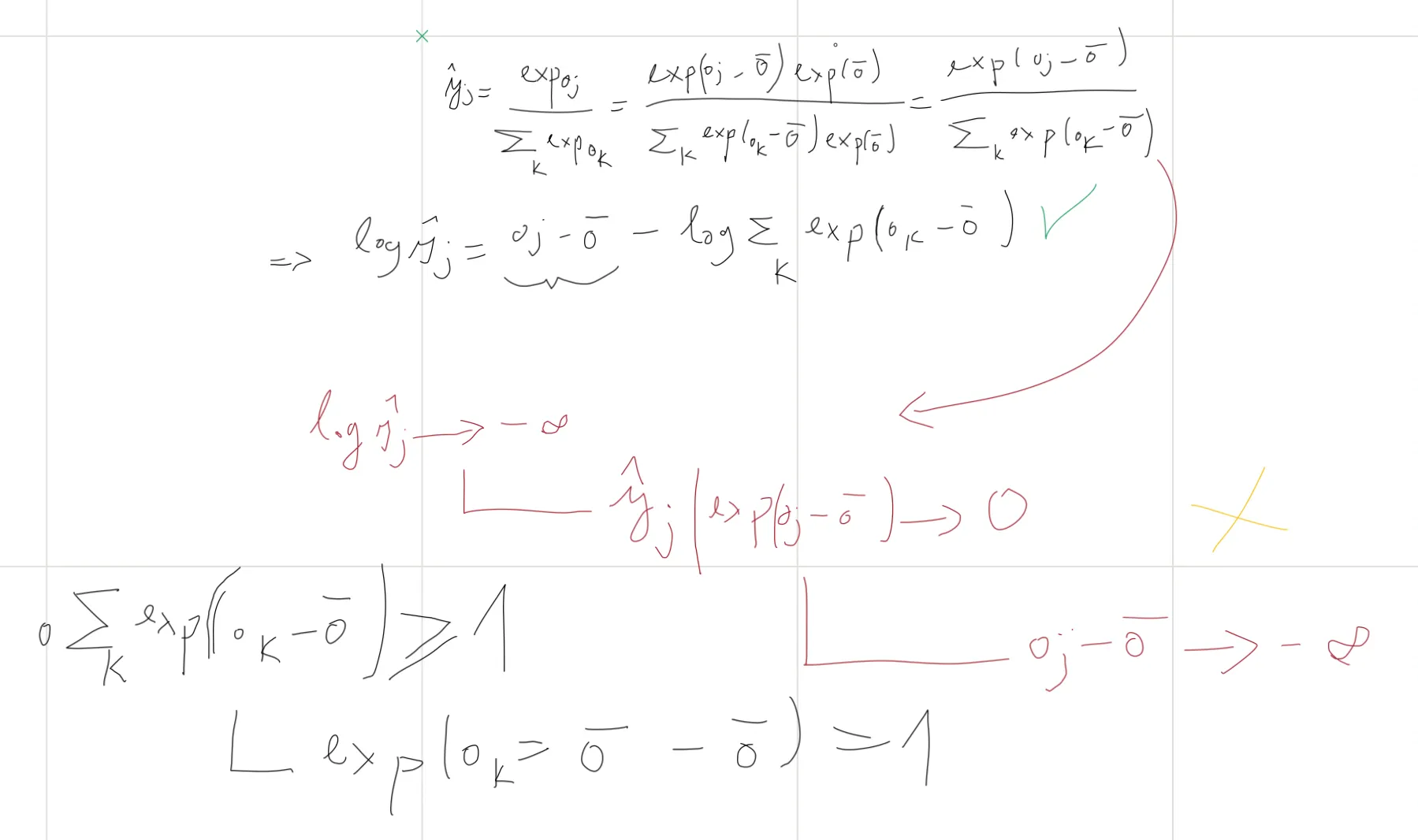
1. Preventing Overflow: Subtracting the Max Logit ()
To stop numbers from blowing up to , we subtract the maximum logit from every score before exponentiating:
Because every power is now :
- The largest exponent is , and all other terms are . Overflow is completely eliminated!
- The denominator , so dividing by zero is impossible.
- Subtracting a constant leaves probabilities unchanged because cancels out in the fraction:
2. Why Underflow Still Causes NaN (The Example)
Subtracting fixes overflow, but creates an underflow trap when calculating loss:
Imagine our model outputs three raw scores: . The maximum is .
- Subtracting max:
- Taking the exponent: For the second class, : Because is far smaller than float32’s minimum limit (), the CPU/GPU forces it to exact .
- The Softmax output:
- The Disaster in Cross-Entropy Loss: If class 2 happens to be the true label (), our loss function evaluates:
- The
NaNContagion in Backpropagation: During gradient descent, calculating gradients with infinity produces undefined arithmetic like or . In computer hardware (IEEE 754), these operations yieldNaN(Not a Number). Once a single weight turns intoNaN, it spreads exponentially across the entire network in the next iteration, destroying the model.
3. The Solution: The LogSumExp Trick
To prevent tiny probabilities from rounding to and blowing up into , we never calculate Softmax first and then take its separately.
Instead, we combine and algebraically into a single stable formula:
Now, re-evaluating our example with class 2 ():
- remains a normal, valid float (never rounded to ).
- .
- The final log probability is:
No , no infinity, and zero NaNs!
Implementing Stable Log-Softmax (LogSumExp) in PyTorch
Here is how we implement the numerically stable Log-Softmax operation using the LogSumExp trick from scratch:
import torch

def log_exp_softmax(outputs: torch.Tensor) -> torch.Tensor:
    # 1. Get max logit per sample (.values extracts tensor from namedtuple)
    max_outputs = outputs.max(dim=1, keepdim=True).values
    # 2. Subtract max to prevent overflow: exp(o - o_max)
    outputs_exp = torch.exp(outputs - max_outputs)
    # 3. Sum the exponentials along class dimension
    partition = outputs_exp.sum(dim=1, keepdim=True)
    # 4. Compute (o - o_max) - log(sum)
return (outputs - max_outputs) - torch.log(partition)PyTorch Built-in (F.log_softmax):
PyTorch implements this exact LogSumExp stabilization under the hood via torch.nn.functional.log_softmax:
import torch.nn.functional as F

# Numerically stable log probabilities
log_probs = F.log_softmax(outputs, dim=1)
In practice, torch.nn.CrossEntropyLoss directly combines log_softmax and nll_loss (Negative Log-Likelihood) into a single, high-performance C++/CUDA kernel.
Implementing Standard Softmax in PyTorch
Here is how we implement the Softmax operation from scratch:
import torch

def softmax(outputs: torch.Tensor) -> torch.Tensor:
    # 1. Exponentiate logits to make them strictly positive
    outputs_exp = torch.exp(outputs)
    # 2. Sum along class dimension (keepdim=True keeps shape (B, 1) for broadcasting)
    partition = outputs_exp.sum(dim=1, keepdim=True)
    # 3. Normalize so each row sums to 1
return outputs_exp / partitionPyTorch Built-in (F.softmax):
PyTorch provides an optimized, numerically stable version via torch.nn.functional.softmax:
import torch.nn.functional as F

# Normalizes along dimension 1 (across all classes for each sample)
probs = F.softmax(outputs, dim=1)
5. Cross-Entropy Loss
How do we measure how good our predicted probabilities are compared to the true label ?
Given a dataset of examples, we want to maximize the probability that our model assigns to the true classes:
Multiplying thousands of small probabilities together quickly causes numerical underflow, and products are hard to differentiate. Instead, we use the natural logarithm .
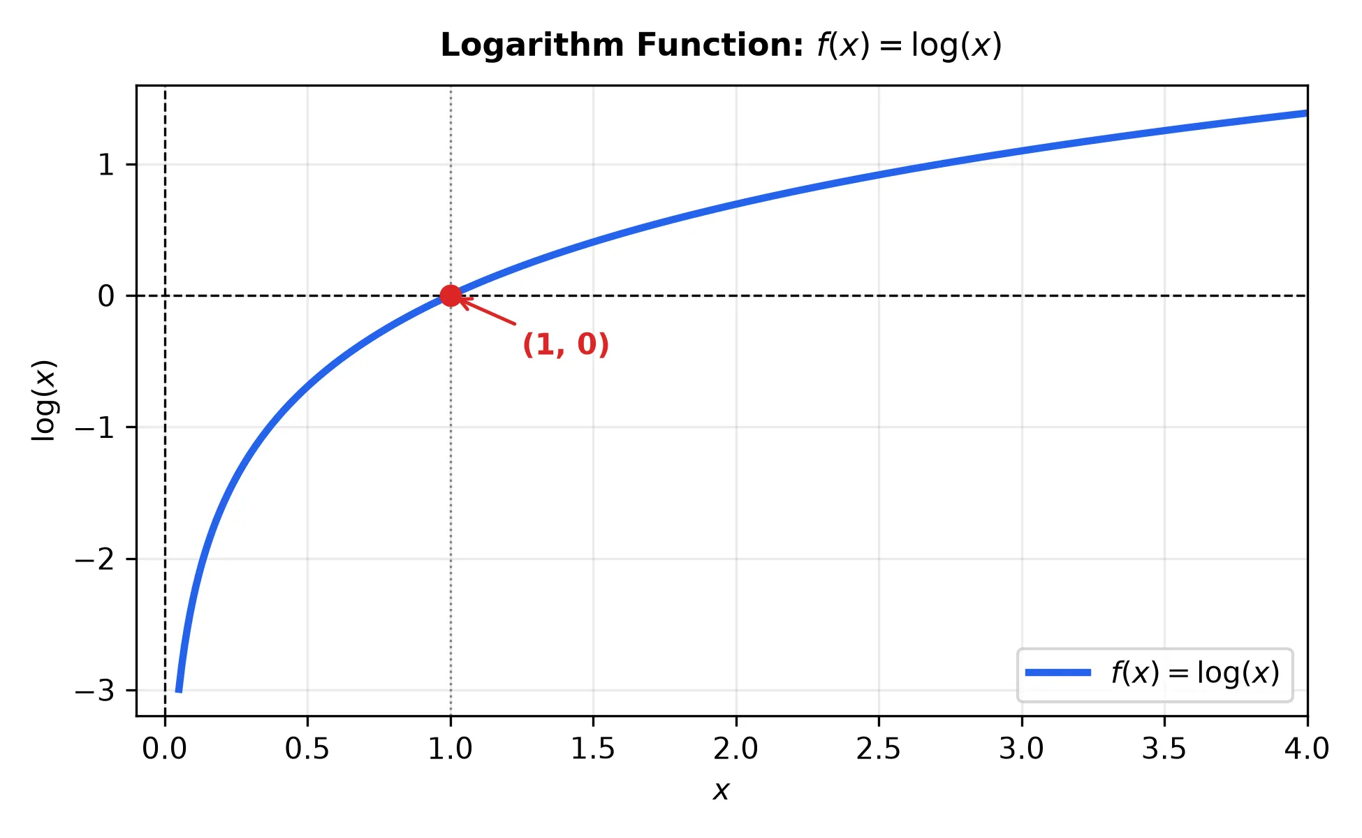
Because probabilities lie between and , is always negative or zero () on . By adding a minus sign — taking the negative logarithm — we flip the values to be positive and turn maximizing probability into minimizing loss:
For a single pair of true one-hot label and predicted probabilities over classes, this gives the Cross-Entropy Loss:
Why Negative Log Works So Intuitively
Since is a one-hot vector (only one and all other ), the entire sum collapses to just the true class :
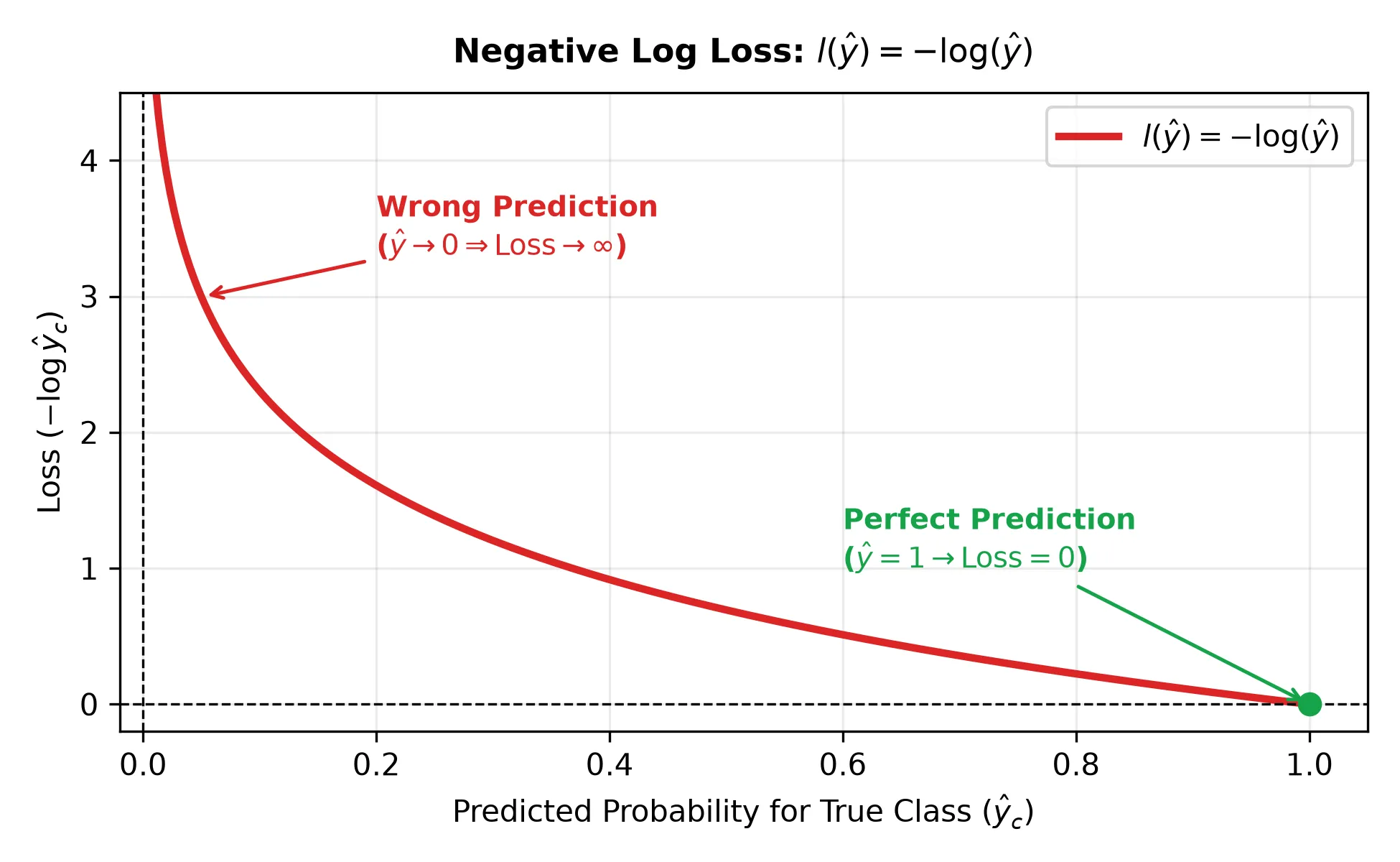
- If (Confident & Correct): . The loss is zero!
- If (Confident & Wrong): . The model gets heavily penalized!
Implementing Cross-Entropy Loss and Training Step in PyTorch
Given the stable log-probabilities from log_exp_softmax, we compute Cross-Entropy Loss using advanced indexing directly with integer target labels (without needing manual one-hot encoding):
import torch

def loss(self, y_hat: torch.Tensor, y: torch.Tensor) -> torch.Tensor:
    # y_hat is log-probabilities from log_exp_softmax
    # -y_hat[range(len(y)), y] extracts the negative log probability of the true class
    return -y_hat[range(len(y)), y].mean()

def training_step(self, batch: tuple[torch.Tensor, torch.Tensor]) -> torch.Tensor:
    X, y = batch
    outputs = self.forward(X)
return self.loss(self.log_exp_softmax(outputs), y)PyTorch Built-in (F.nll_loss / nn.CrossEntropyLoss):
- Because
log_exp_softmaxalready computes log-probabilities , passing them to PyTorch’s Negative Log-Likelihood lossF.nll_lossgives the exact same result:loss = F.nll_loss(log_probs, y) - In standard PyTorch workflows,
torch.nn.CrossEntropyLoss()combineslog_softmaxandnll_lossdirectly from raw logits in one optimized step:criterion = torch.nn.CrossEntropyLoss() loss = criterion(outputs, y)
6. Softmax and Cross-Entropy Gradient
To train our model with Gradient Descent, we need the derivative of the Cross-Entropy loss with respect to each raw logit .
Quick Calculus Recall (Logarithm Rules):
- Quotient Rule for Logs:
- Log of Exponential:
- Derivative of Natural Log:
- Chain Rule with Log:
Let’s plug the Softmax formula into the Cross-Entropy loss and simplify step-by-step:
Since is a one-hot vector, the sum of all its elements is . This simplifies the loss to:
Now, taking the derivative with respect to a specific logit using the chain rule :
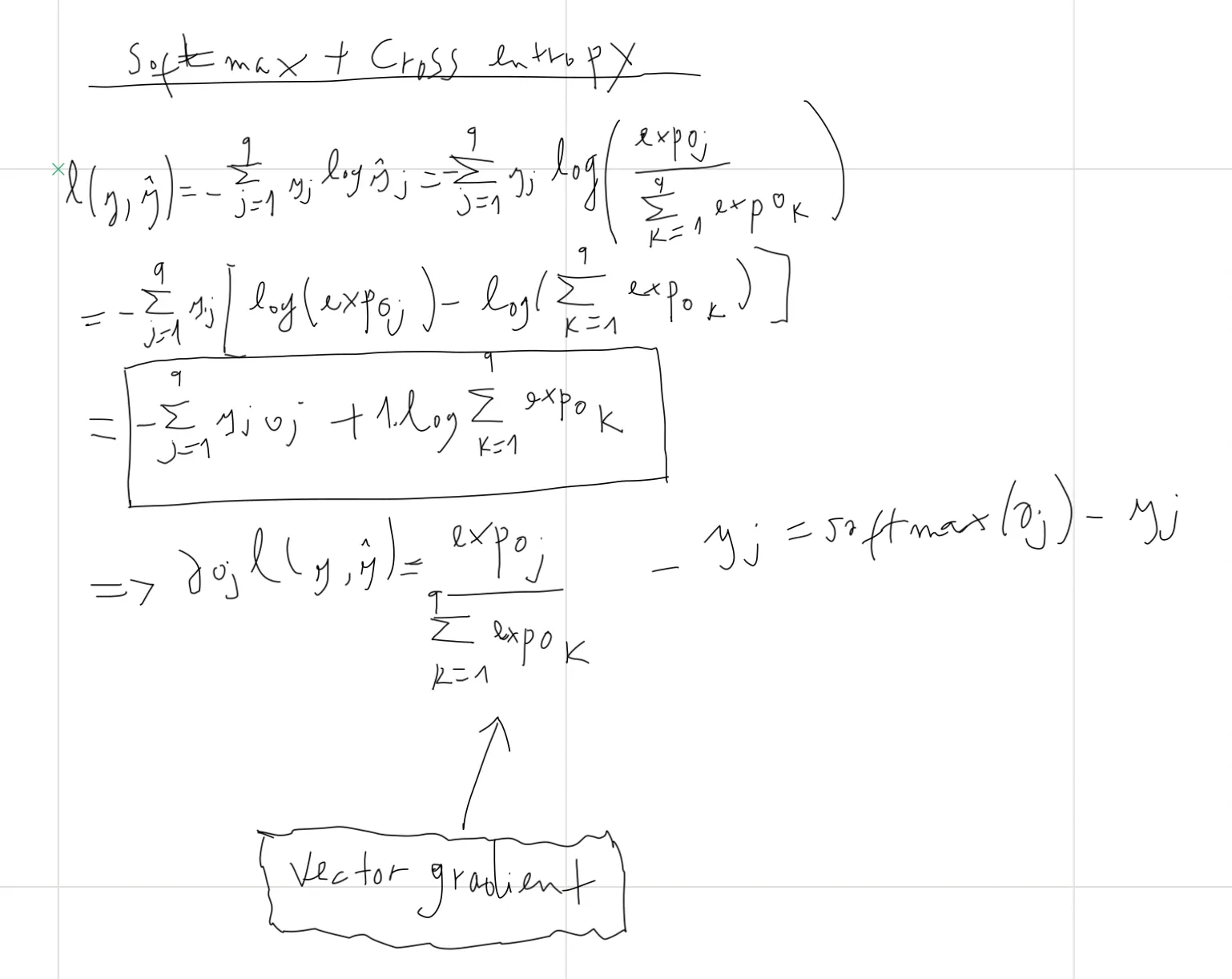
The Beauty of This Result: The gradient is simply Prediction minus Truth — the exact same form as Linear Regression! If our model predicts for the true class (), the gradient is , gently nudging the weight to increase that score.
7. Putting It All Together: Complete PyTorch Pipeline
Here is the complete, self-contained implementation from scratch — combining data loading, model architecture, stable Log-Softmax, Cross-Entropy Loss, custom SGD optimizer, and the training loop:
import matplotlib.pyplot as plt
import torch
from torchvision import datasets, transforms


def show_images(imgs, num_rows, num_cols, titles=None, scale=1.5, save_path=None):
    figsize = (num_cols * scale, num_rows * scale)
    fig, axes = plt.subplots(num_rows, num_cols, figsize=figsize)
    if num_rows * num_cols == 1:
        axes = [axes]
    else:
        axes = axes.flatten()

    for i, (ax, img) in enumerate(zip(axes, imgs)):
        if isinstance(img, torch.Tensor):
            img = img.detach().cpu().numpy()

        if img.ndim == 3:
            if img.shape[0] == 1:
                img = img.squeeze(0)
            elif img.shape[0] == 3:
                img = img.transpose(1, 2, 0)

        cmap = "gray" if img.ndim == 2 else None
        ax.imshow(img, cmap=cmap)
        ax.axis("off")
        if titles is not None and i < len(titles):
            ax.set_title(titles[i], fontsize=10)

    plt.tight_layout()
    if save_path:
        plt.savefig(save_path, bbox_inches="tight")
    else:
        plt.show()
    return axes


class FashionMNIST:
    def __init__(self, batch_size=64, resize=(28, 28), root="./data", num_workers=4):
        self.batch_size = batch_size
        self.resize = resize
        self.root = root
        self.num_workers = num_workers
        trans = transforms.Compose([transforms.Resize(resize), transforms.ToTensor()])
        self.train = datasets.FashionMNIST(
            root=self.root, train=True, transform=trans, download=True
        )
        self.val = datasets.FashionMNIST(
            root=self.root, train=False, transform=trans, download=True
        )

    def text_labels(self, indices):
        labels = [
            "t-shirt", "trouser", "pullover", "dress", "coat",
            "sandal", "shirt", "sneaker", "bag", "ankle boot"
        ]
        return [labels[int(i)] for i in indices]

    def get_data_loader(self, train):
        data = self.train if train else self.val
        return torch.utils.data.DataLoader(
            data, self.batch_size, shuffle=train, num_workers=self.num_workers
        )

    def visualize(self, batch, nrows=1, ncols=8, labels=None, save_path=None):
        X, y = batch
        n = nrows * ncols
        imgs = X[:n]
        if labels is None:
            lbls = self.text_labels(y[:n])
        else:
            lbls = labels[:n]
        return show_images(imgs, nrows, ncols, titles=lbls, save_path=save_path)


class ClassificationModel:
    def __init__(
        self,
        num_features: int,
        num_classes: int,
        learning_rate: float = 0.1,
        sigma: float = 0.01,
    ):
        self.num_features = num_features
        self.learning_rate = learning_rate
        self.W = torch.normal(
            0, sigma, (num_features, num_classes), dtype=torch.float32, requires_grad=True
        )
        self.b = torch.zeros(num_classes, dtype=torch.float32, requires_grad=True)
        self.params = [self.W, self.b]

    def forward(self, X: torch.Tensor) -> torch.Tensor:
        X = X.reshape(-1, self.num_features)
        return torch.matmul(X, self.W) + self.b

    def log_exp_softmax(self, outputs: torch.Tensor) -> torch.Tensor:
        output_max = outputs.max(dim=1, keepdim=True).values
        output_exp = torch.exp(outputs - output_max)
        sum_exp = output_exp.sum(dim=1, keepdim=True)
        return outputs - output_max - torch.log(sum_exp)

    def loss(self, y_hat: torch.Tensor, y: torch.Tensor) -> torch.Tensor:
        return -y_hat[range(len(y)), y].mean()

    def training_step(self, batch: tuple[torch.Tensor, torch.Tensor]) -> torch.Tensor:
        X, y = batch
        outputs = self.forward(X)
        return self.loss(self.log_exp_softmax(outputs), y)


class SGD:
    def __init__(self, params: list[torch.Tensor], learning_rate: float):
        self.params = params
        self.learning_rate = learning_rate

    def step(self):
        with torch.no_grad():
            for param in self.params:
                if param.grad is not None:
                    param -= self.learning_rate * param.grad

    def zero_grad(self):
        for param in self.params:
            if param.grad is not None:
                param.grad.zero_()


def evaluate_accuracy(model: ClassificationModel, data_loader) -> float:
    correct_count = 0
    total_count = 0
    with torch.no_grad():
        for X, y in data_loader:
            outputs = model.forward(X)
            predictions = outputs.argmax(dim=1)
            correct_count += (predictions == y).sum().item()
            total_count += y.shape[0]
    return correct_count / total_count


if __name__ == "__main__":
    data = FashionMNIST(batch_size=64, resize=(28, 28), root="./data")
    train_loader = data.get_data_loader(train=True)
    val_loader = data.get_data_loader(train=False)

    model = ClassificationModel(
        num_features=28 * 28, num_classes=10, learning_rate=0.1
    )
    optimizer = SGD(model.params, learning_rate=model.learning_rate)
    num_epochs = 5

    print("Starting training...")
    for epoch in range(num_epochs):
        total_loss = 0.0
        num_batches = 0

        for batch in train_loader:
            optimizer.zero_grad()
            loss = model.training_step(batch)
            loss.backward()
            optimizer.step()

            total_loss += loss.item()
            num_batches += 1

        val_accuracy = evaluate_accuracy(model, val_loader)
        average_loss = total_loss / num_batches
        print(
            f"Epoch {epoch + 1}/{num_epochs} | Loss: {average_loss:.4f} | Validation Accuracy: {val_accuracy * 100:.2f}%"
        )
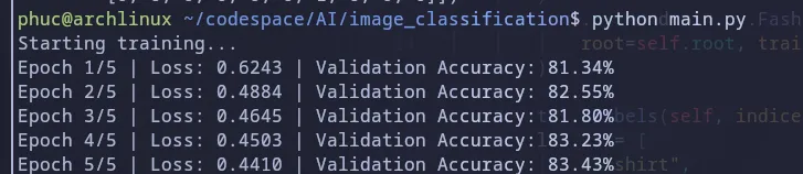
Training Results
Training our scratch model for 5 epochs steadily drives loss down from 0.6243 to 0.4410, reaching 83.43% Validation Accuracy:
Interpreting the Model: Learned Weight Templates
A linear model cannot understand complex shapes or real spatial depth. So why does it still reach ~84% accuracy?
Under the hood, it performs Template Matching:
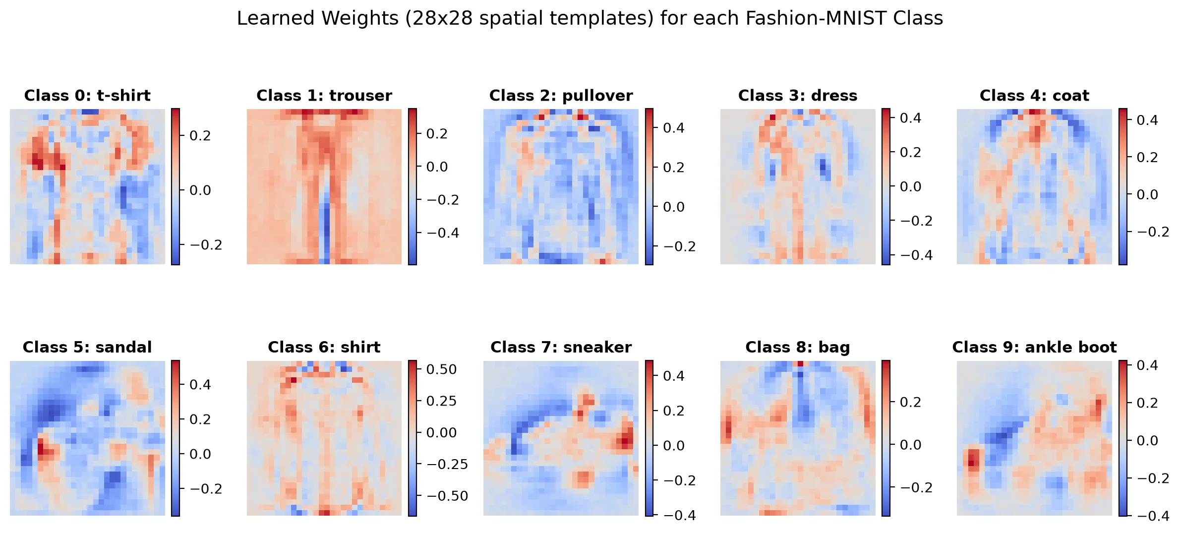
- Each class learns an average template: Reshaping each weight column back to reveals a ghostly “prototype” image of that category.
- Positive weights (, Red): Positions where the item usually has bright pixels (like the two trouser legs or the sole of a sneaker). Matching pixels here boost the class score.
- Negative weights (, Blue): Positions that must remain dark (like the empty space between two trouser legs). Bright pixels here heavily penalize the score.
- Classification by overlay: The model simply overlays the input image onto all 10 templates. Whichever template has the strongest overlap (highest dot product ) wins!
This works surprisingly well on Fashion-MNIST because all images are cleanly normalized: centered, identical in size, and viewed from the exact same angle.
8. Conclusion
- Regression vs. Classification: Regression predicts “How much?” (1 output); Classification predicts “Which category?” ( outputs).
- One-Hot Encoding: Represents unordered categories without introducing fake numerical distances.
- Softmax: Converts unconstrained linear scores (logits) into positive probabilities that sum to .
- Cross-Entropy Loss: Measures the negative log probability of the true class (), heavily punishing confident wrong predictions.
- Simple Gradient: Combining Softmax and Cross-Entropy yields the clean gradient .