What is a Neural Network?

This blog will briefly introduce the core concepts of Neural Networks.

Table of contents

What is the Neural Network?

On the surface, a machine recognizing handwritten digits seems not an impressive task at all. I bet you can tell that these are all images of the digit three:

• Each “three” is drawn differently, yet you can somehow easily recognize it. But if I told you to sit down and write a program that takes in a grid of 28x28 pixels and outputs a single number between 0 and 9, the task goes from easy to extremely difficult.

• Somehow, identifying digits is incredibly easy for your brain to do, but almost impossible for you to describe how you do it. Furthermore, traditional methods of computer programming—with normal loops, classes, objects, and functions—don’t seem suitable to tackle this problem.

• But what if we could write a program that mimics the structure of your brain? That’s exactly the core idea behind neural networks.

The Structure of a Neural Network

An Artificial Neural Network (ANN) is composed of interconnected units called neurons (or nodes) organized into distinct layers:

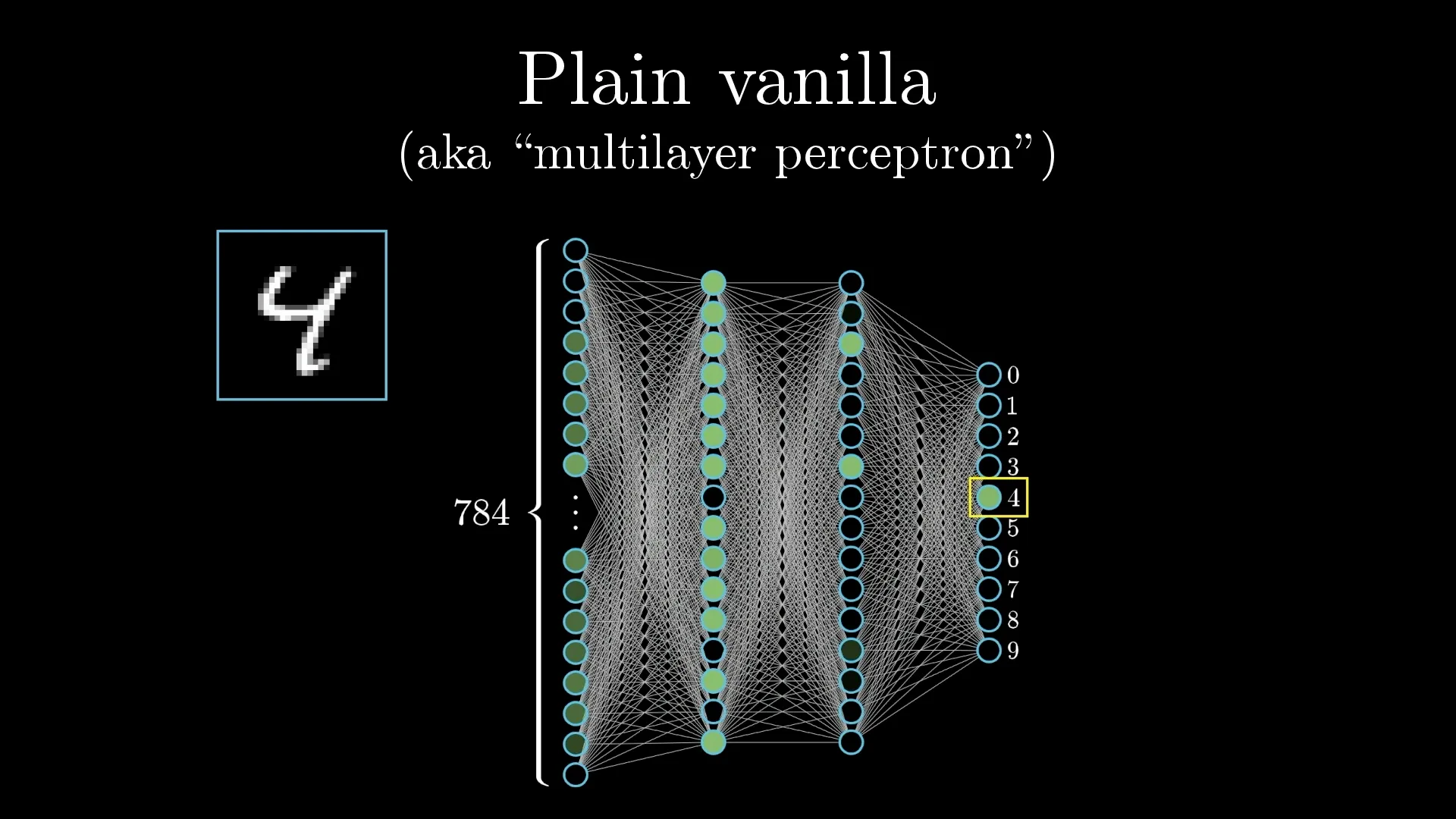Figure 1: A multilayer neural network with 784 input neurons, two hidden layers of 16 neurons each, and 10 output neurons (Inspired by 3Blue1Brown).

1. Neurons & Activations

• A neuron is a container holding a single number, known as its activation value (typically ranging from 0.0 to 1.0).
• Higher activation means the neuron is strongly “lit up” or firing.

2. The Three Types of Layers

1. Input Layer:
   • Receives raw data from the outside world.
   • For our 28x28 pixel digit image, the input layer consists of 784 neurons (28 x 28 = 784), where each neuron’s activation corresponds to the brightness of a single pixel.

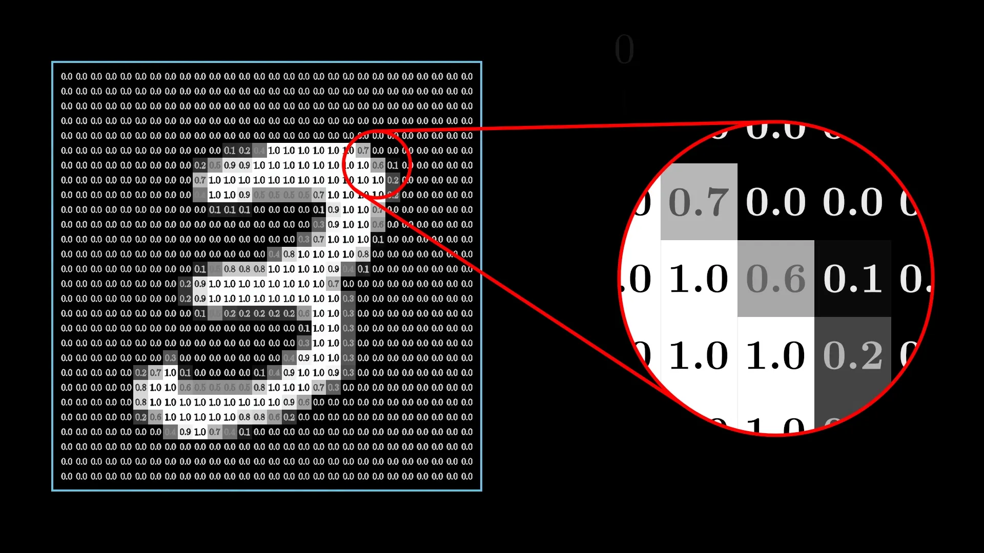Each pixel’s brightness (0.0 = black, 1.0 = white) becomes one neuron’s activation in the input layer.

2. Hidden Layers:
   • Located between the input and output layers.
   • These layers break down complex tasks into sub-patterns hierarchically:
     • Layer 1: Detects small, simple line segments and edges.
     • Layer 2: Combines edges into sub-components like loops, strokes, or arcs (e.g., the top loop of a 3).

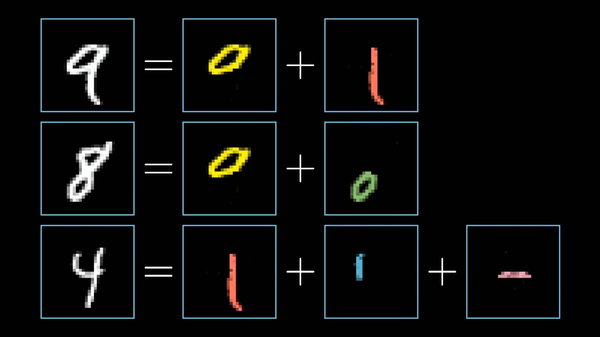Figure 2: Hidden layers assemble low-level features (edges & lines) into high-level shapes (loops & components).

3. Output Layer:
   • Provides the final answer.
   • Consists of 10 neurons representing the digits 0 through 9. The neuron with the highest activation score is the network’s final prediction!

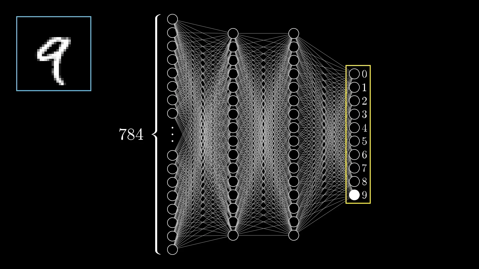The output layer lights up neuron “9” — the network’s confident prediction for this handwritten digit.

3. How Neurons Connect: Weights & Biases

Information flows through connections between neurons:

• Weights ($w$): Every connection has an assigned weight—a number indicating how strongly one neuron influences another. Positive weights excite target neurons, while negative weights inhibit them.
• Biases ($b$): An extra offset added to each neuron to control its threshold for activation (how easily it fires).

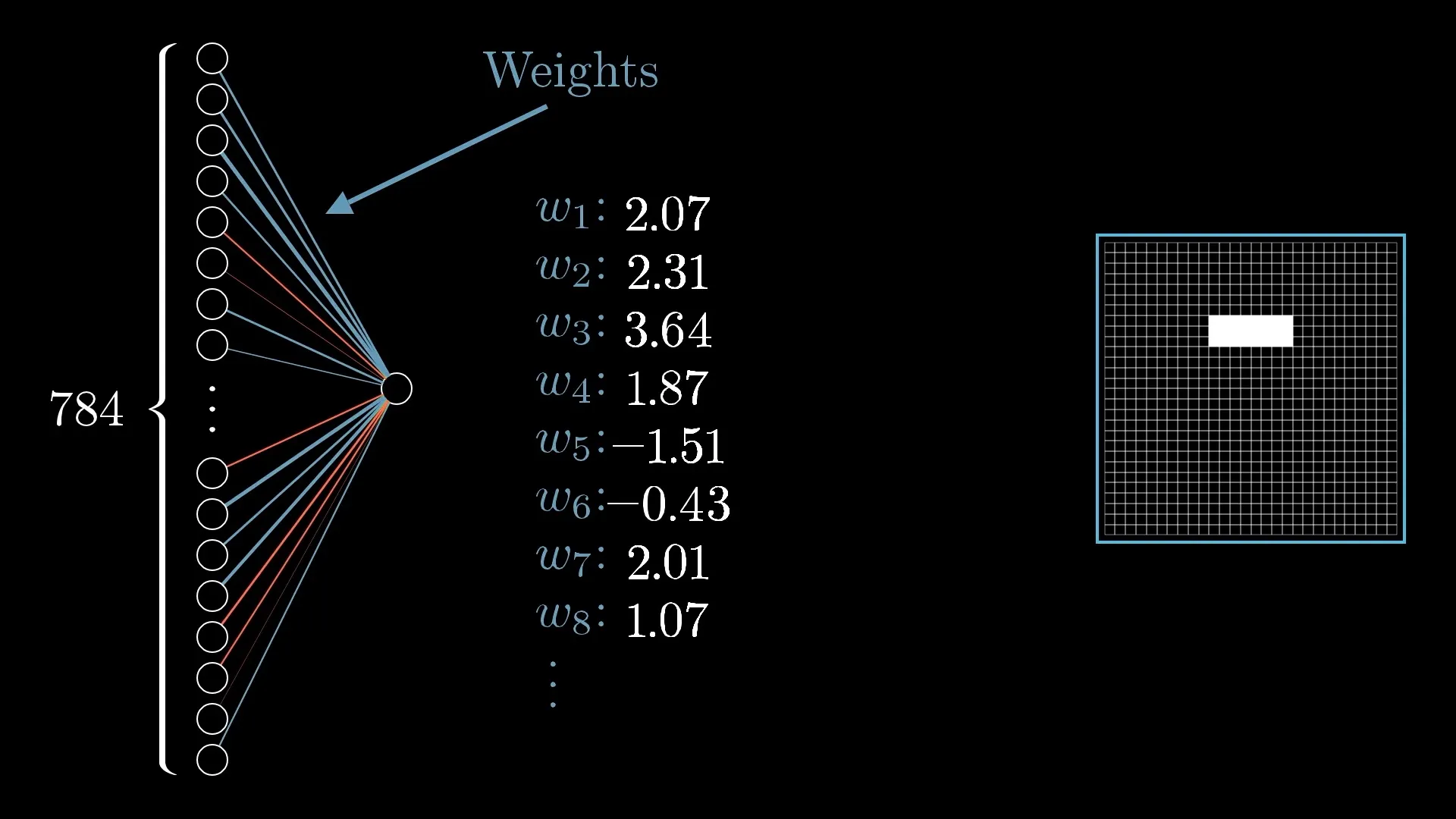Weights dictate the strength and sign of connections between neurons, while biases tune their activation thresholds.

How a Neuron Computes its Output

Each neuron calculates a weighted sum of its inputs plus a bias:

Then, it passes this result through an activation function (such as Sigmoid or ReLU) to compress the output into a normalized range (0.0 to 1.0) and introduce non-linearity.

The Sigmoid Activation Function ($\sigma$)

The Sigmoid function is a mathematical function defined as:

• Squashing Inputs: It squashes any real-valued weighted input $z$ into a normalized activation range between 0.0 and 1.0.
• Behavior: Extremely high values approach 1.0 (strongly firing neuron), extremely low negative values approach 0.0 (inactive neuron), and $x = 0$ outputs 0.5.

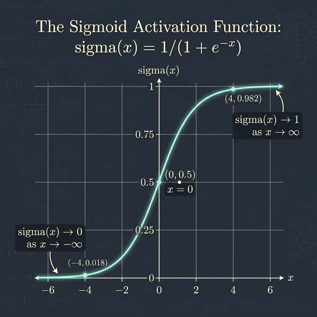The Sigmoid S-curve squashes raw weighted sums into valid activation scores between 0 and 1.

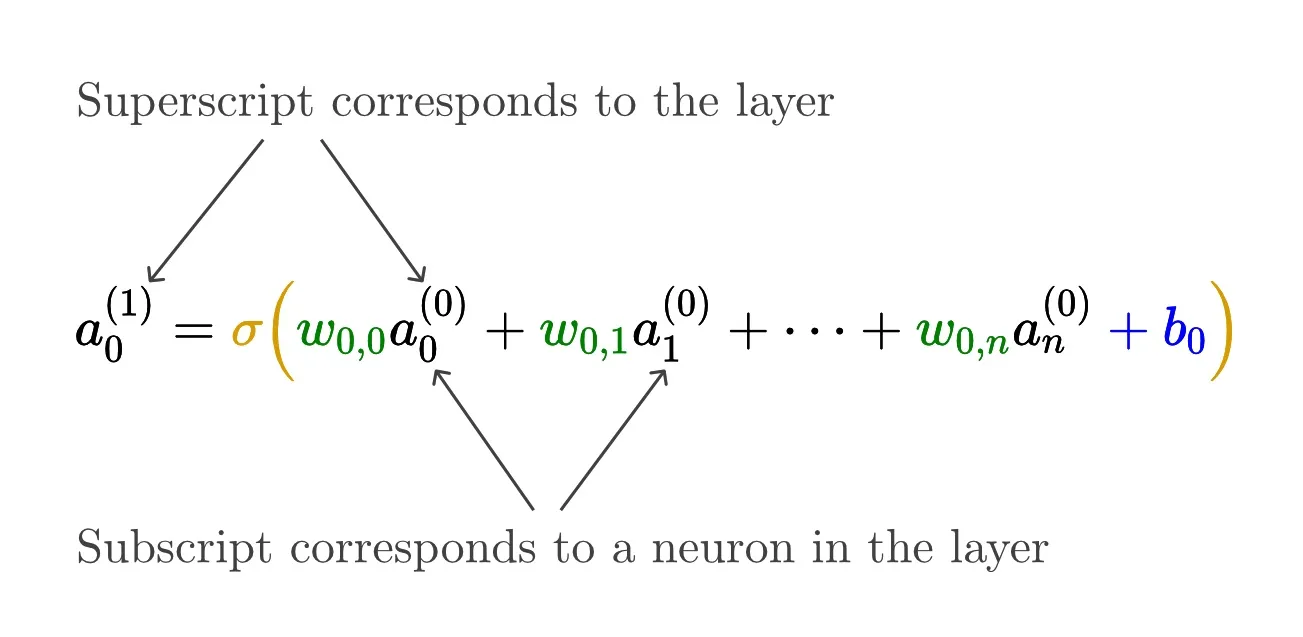Figure 3: Vectorized layer equation $a^{(1)} = \sigma(W a^{(0)} + b)$ representing all weights, activations, and biases across a layer.

How Information Passes Between Layers

Information in a neural network flows sequentially forward from layer to layer (Forward Propagation):

• Activation Cascade: The activations $a^{(L-1)}$ from layer $L-1$ act as inputs to calculate the activations $a^{(L)}$ of layer $L$.
• Weighted Influence: Each connection carries a weight $w$ that dictates how much the previous neuron excites or suppresses the next neuron.
• Matrix Computation: Rather than calculating neuron by neuron, an entire layer’s activations are computed at once using matrix operations:

Where $W^{(L)}$ is the weight matrix, $b^{(L)}$ is the bias vector, and $\sigma$ is the activation function.

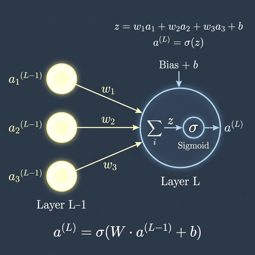Figure 4: How activations flow from layer $L-1$ through weighted sum and activation function $\sigma$ to produce activations for layer $L$.

How Neural Networks Learn 🎯

A brand-new neural network starts with completely random weights and biases—meaning its initial guesses are pure garbage!

Learning happens through a 3-step loop:

1. Forward Propagation: Pass the input image through the network to compute a prediction.
2. Loss Calculation: Compare the prediction with the true label to calculate the Cost / Loss (how wrong the network was).
3. Backpropagation & Optimization: Use gradient descent to tweak every weight and bias slightly to reduce the error on the next try.

Repeat this process over thousands of training examples, and the network gradually learns to recognize digits with remarkable accuracy!