Backpropagation Calculus

This post covers the mathematical foundation of Backpropagation Calculus, explaining step-by-step how gradients flow backwards through a neural network using the multivariable chain rule.

Table of contents

What is Backpropagation Calculus?

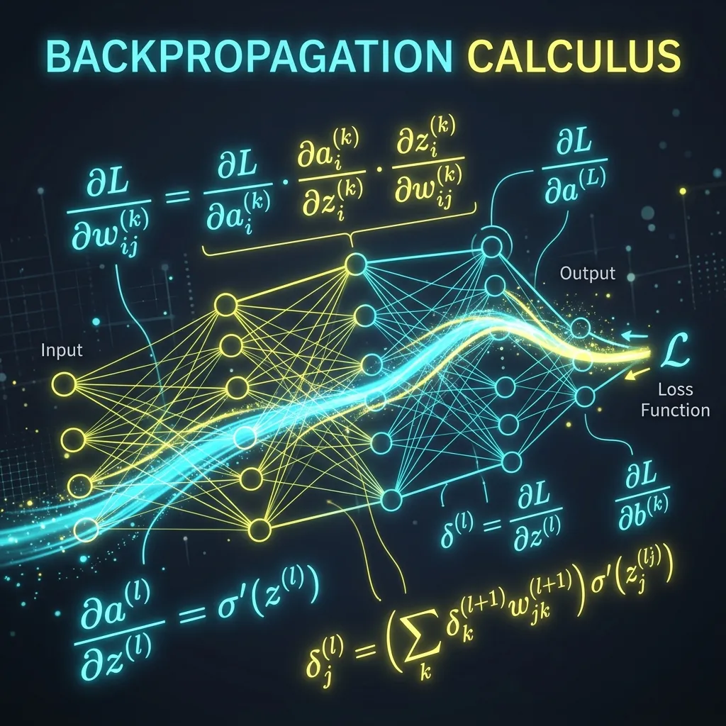
Backpropagation is the foundational algorithm that computes the gradient of the cost function $\nabla C$. The entries of this gradient vector represent the partial derivatives of the cost function $C$ with respect to every weight ($w$) and bias ($b$) throughout the network:

Calculating these partial derivatives quantifies how sensitive the network’s total error is to small perturbations in each parameter, enabling Gradient Descent to systematically update parameters in the direction of steepest descent: $w \leftarrow w - \alpha \frac{\partial C}{\partial w}$ (where $\alpha$ is the learning rate).

1. Simple Case: One Neuron per Layer

To understand the calculus intuitively, consider a simplified network where each layer contains a single neuron.

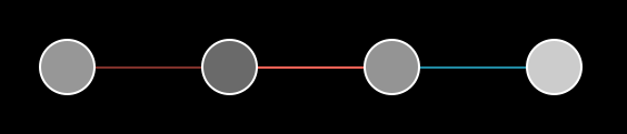Figure 1: A simplified neural network architecture with one neuron per layer.

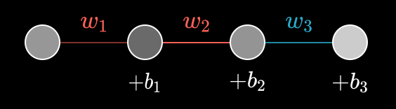Figure 2: Parameters ($w$ and $b$) defining connections and activation thresholds between consecutive neurons.

For a single training sample with desired target output $y$:

• Weighted Input: $z^{(L)} = w^{(L)} a^{(L-1)} + b^{(L)}$
• Activation Output: $a^{(L)} = \sigma(z^{(L)})$ (where $\sigma$ is the activation function)
• Sample Cost: $C_0 = (a^{(L)} - y)^2$ (the squared error loss)

The Chain Rule Breakdown

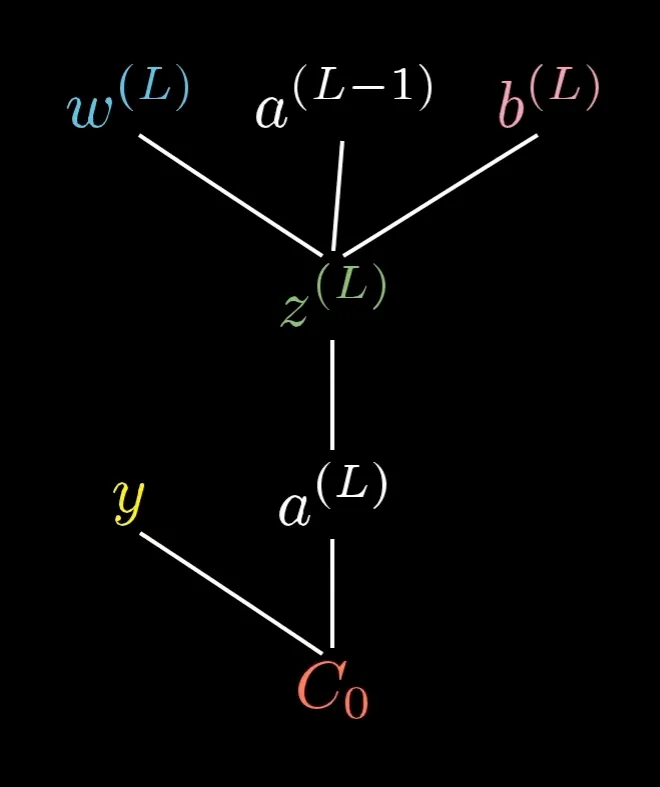Figure 3: Computational dependency graph illustrating how $w^{(L)}, b^{(L)}, a^{(L-1)}$ determine $z^{(L)}$, which computes activation $a^{(L)}$, ultimately yielding cost $C_0$.

To determine how a small change in weight $w^{(L)}$ impacts the cost $C_0$, we apply the Multivariable Chain Rule:

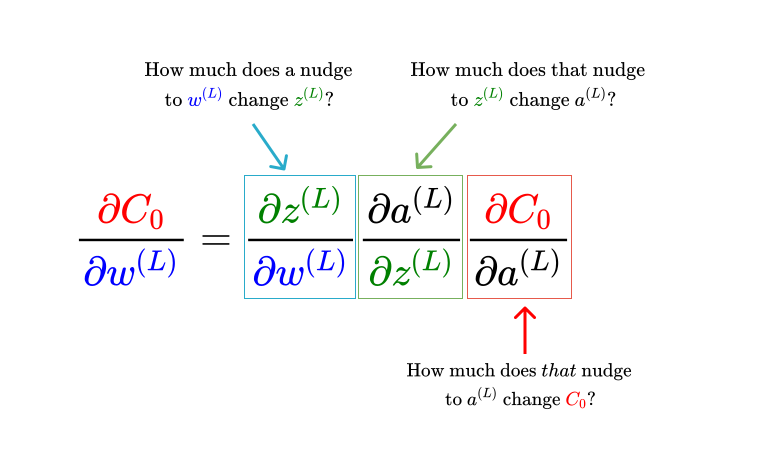Figure 4: Decomposing the partial derivative $\frac{\partial C_0}{\partial w^{(L)}}$ into three constituent derivative ratios.

Computing the Three Factors

1. Previous Activation Sensitivity:

   $$\frac{\partial z^{(L)}}{\partial w^{(L)}} = a^{(L-1)}$$

   (Reflects Hebbian learning: higher activation $a^{(L-1)}$ amplifies the weight change’s effect on the weighted input).

2. Activation Function Gradient:

   $$\frac{\partial a^{(L)}}{\partial z^{(L)}} = \sigma'(z^{(L)})$$

   (Measures the local derivative/slope of the non-linear activation function).

3. Output Error Sensitivity:

   $$\frac{\partial C_0}{\partial a^{(L)}} = 2(a^{(L)} - y)$$

   (Proportional to the raw prediction error; larger errors induce steeper gradient updates).

Combining the Partial Derivatives

Multiplying these three factors yields the exact sensitivity for a single weight:

Similarly, for the bias $b^{(L)}$, since $\frac{\partial z^{(L)}}{\partial b^{(L)}} = 1$:

2. Propagating Backwards to Hidden Layers

To compute gradients for parameters in earlier hidden layers (e.g., $w^{(L-1)}$), we first evaluate the cost’s sensitivity to the previous activation $a^{(L-1)}$:

By computing $\frac{\partial C_0}{\partial a^{(L-1)}}$, we backward propagate the error signal layer-by-layer, efficiently evaluating derivatives for all preceding weights and biases.

3. Cost Over All Training Examples

The overall cost function $C$ across a full dataset of $n$ samples is the arithmetic mean:

By the linearity of differentiation, the derivative of total cost $C$ with respect to any parameter is the average of individual sample derivatives:

4. Generalizing to Multineuron Layers

In a general deep network with multiple neurons per layer:

• $a_k^{(L-1)}$: Activation of neuron $k$ in layer $L-1$.
• $a_j^{(L)}$: Activation of neuron $j$ in layer $L$.
• $w_{jk}^{(L)}$: Weight connecting neuron $k$ in layer $L-1$ to neuron $j$ in layer $L$.

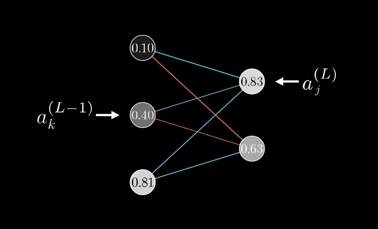Figure 5: Indexing activations $a_k^{(L-1)}$ and $a_j^{(L)}$ alongside weight matrix entry $w_{jk}^{(L)}$ across dense layers.

The weighted sum $z_j^{(L)}$ for neuron $j$ is:

Multiple Paths of Computational Influence

In fully connected layers, a single neuron $k$ in layer $L-1$ influences every neuron $j$ in layer $L$. Consequently, changing $a_k^{(L-1)}$ affects the cost through multiple computation paths. By multivariate calculus, we sum the chain rule across all output neurons in layer $L$:

Conclusion

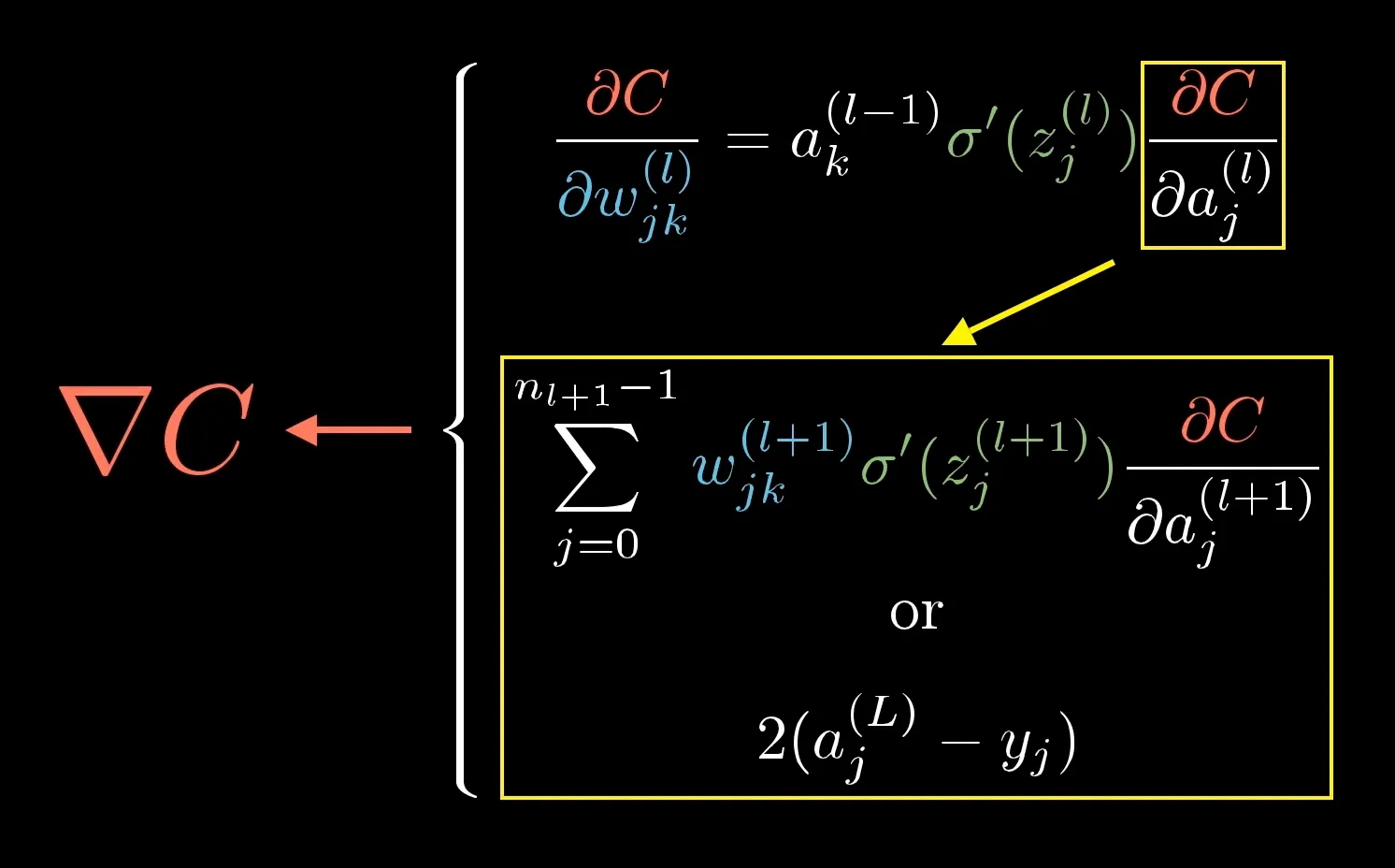Figure 6: Complete mathematical summary of backpropagation calculus formulas across layers.

Backpropagation boils down to three core principles:

1. Chain Rule Engine: Applies the multivariable chain rule to calculate how sensitive the cost function is to every weight and bias.
2. Backward Error Flow: Computes error signals starting from the output layer and propagates them backward through hidden layers.
3. Vectorized Optimization: Aggregates partial derivatives into a gradient vector ($\nabla C$), enabling modern frameworks to update parameters efficiently using Gradient Descent.