In Machine Learning, getting 100% accuracy on your training data is rarely good news. In fact, it is often a warning sign. What really matters is how well your model performs on new, unseen data.
In this article, we break down what generalization really means, what factors control model complexity, how to safely split your data, and how to use K-Fold Cross-Validation.

Table of contents
Open Table of contents
1. Memorization vs. Generalization: The Student Metaphor
Imagine two students preparing for an exam:
- Harry (The Memorizer): Harry has a photographic memory. He memorizes every question and answer key from past exams word-for-word.
- Jack (The Generalizer): Jack has an average memory, but he focuses on understanding the core ideas and problem-solving rules.
What happens on exam day?
| Scenario | Harry’s Score | Jack’s Score |
|---|---|---|
| Old Questions (Repeated from past years) | 100% (Perfect recall) | 90% (A few small slips) |
| New Questions (Brand-new problems) | < 50% (Struggles completely) | 90% (Solves them easily) |
In machine learning, we want our models to be Jack, not Harry. We do not want models that just remember past examples; we want models that discover underlying rules so they can make accurate predictions on future data.
- Underfitting: The model is too simple and didn’t learn enough (Jack didn’t study).
- Overfitting: The model memorized the training data and its random noise (Harry memorizing the answer key).
- Regularization: Techniques we use to stop overfitting and help the model generalize.
2. The Generalization Gap
When training any model, we track two types of errors:
- Training Error: The error on the data the model is currently learning from.
- Generalization Error: The error when the model is tested on new, unseen data (measured using a separate validation or test set).
The difference between these two errors is the Generalization Gap:
Why Low Training Error Can Fool You
Deep neural networks have millions of parameters. With that much capacity, a network can easily memorize every single training sample with training error without understanding the true pattern.
Key takeaway: A low training error does not mean your model works. You must always verify its performance on a separate validation set.
3. Model Complexity
Finding the right model is all about balance — you want a model that is neither too simple nor too complex.
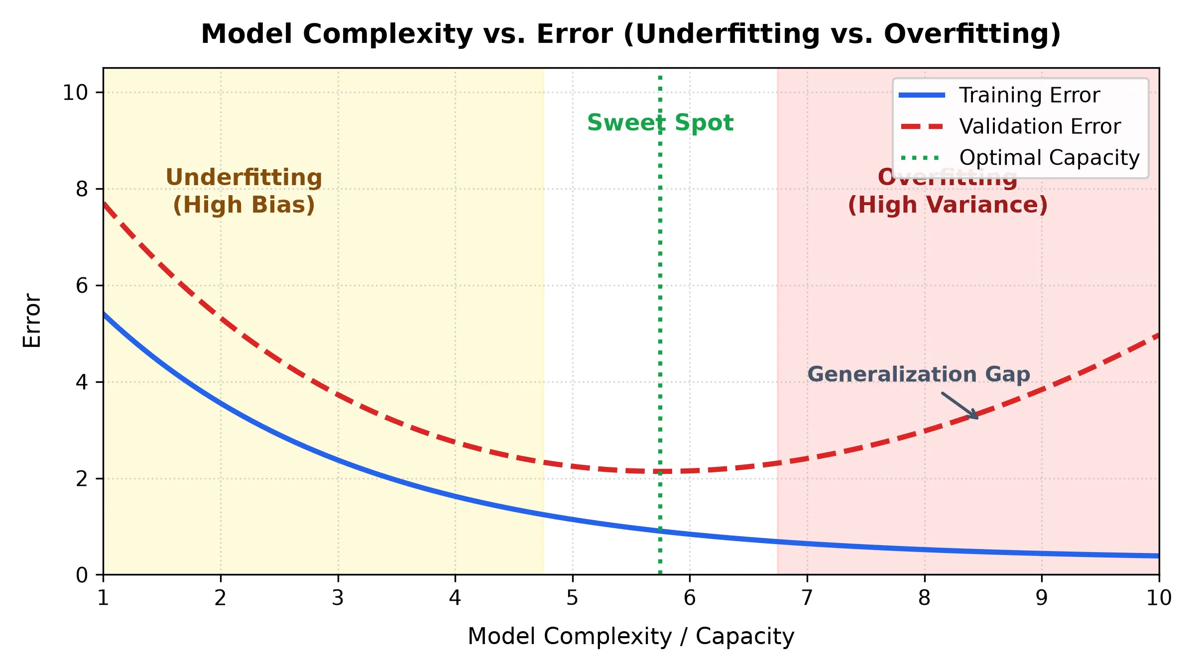
- Too Simple (Underfitting / High Bias): The model does not have enough power to learn the pattern (for example, trying to fit a straight line to a curved relationship). Both training and validation errors stay high.
- Just Right (The Sweet Spot): The model captures the true pattern and ignores random noise. Validation error reaches its lowest point.
- Too Complex (Overfitting / High Variance): The model bends and twists to hit every single training point. Training error drops near , but validation error shoots up, creating a huge generalization gap.
Karl Popper’s Principle of Falsifiability
The philosopher Karl Popper argued that a scientific theory must be falsifiable — if an explanation can fit any outcome (even complete nonsense), it is not scientific.
In Machine Learning:
- If your model is so flexible that it can achieve error even when labels are assigned completely at random, getting on real data proves nothing.
- A reliable model is constrained enough that it fails on random noise, but succeeds on real-world patterns.
4. What Factors Define Model Complexity?
What actually makes a model “simple” or “complex”? It comes down to five key factors:
- Number of Parameters (Weights): More weights give the model more flexibility to curve and bend. A model with 2 weights () can only draw a line. A model with millions of weights can outline almost any shape.
- Size of the Weights (Parameter Range):
Model complexity is not just about the number of weights — it is also about how big those weights are allowed to become.
- If weights can grow huge, tiny changes in input cause wild swings in output (overfitting).
- Restricting weights to remain small keeps the model smooth and well-behaved. This is the exact idea behind Weight Decay ( Regularization):
- Number of Input Features: Feeding raw features () keeps things simple. Adding polynomial features () dramatically increases model complexity.
- Network Depth and Architecture: Adding more layers and non-linear activations increases how complicated of a relationship the network can represent.
- Training Time (Epochs): Training for too many iterations gives the model extra time to start fitting noise in the training set.
5. How Dataset Size Changes the Game
A model’s complexity should always match the size of your dataset:
- Small Datasets (Hundreds to thousands of rows): Simple models (like Linear Regression or Decision Trees) are hard to beat. Deep neural networks have too many parameters for small datasets and will quickly overfit by memorizing the examples.
- Large Datasets (Hundreds of thousands to millions of rows): Simple models hit a wall (underfitting) because they cannot capture intricate relationships. Deep learning models thrive here because big datasets give them enough evidence to learn complex rules without memorizing noise.
Golden Rule: Never increase model complexity faster than your dataset size.
6. Model Selection: The 3-Way Data Split
When developing a machine learning model, you have to make many choices: how many layers to use, which learning rate to set, how much weight decay to apply, and which features to keep. This trial-and-error process is called Model Selection.
To select the best model fairly, you must divide your data into three separate sets:
- Training Set (The Practice Homework): Used by the optimization algorithm (like SGD or Adam) to update weights and biases .
- Validation Set (The Mock Exam): Used by you to compare different models, tune hyperparameters, and check for overfitting.
- Test Set (The Final Exam in a Sealed Vault): Kept completely untouched while you experiment. It is evaluated only once at the very end to give an honest, unbiased score of how the model will perform in the real world.
7. K-Fold Cross-Validation: Safe Validation for Small Data
When you have a small dataset, setting aside 20% to 30% for validation can feel wasteful — you lose precious training data that your model needs.
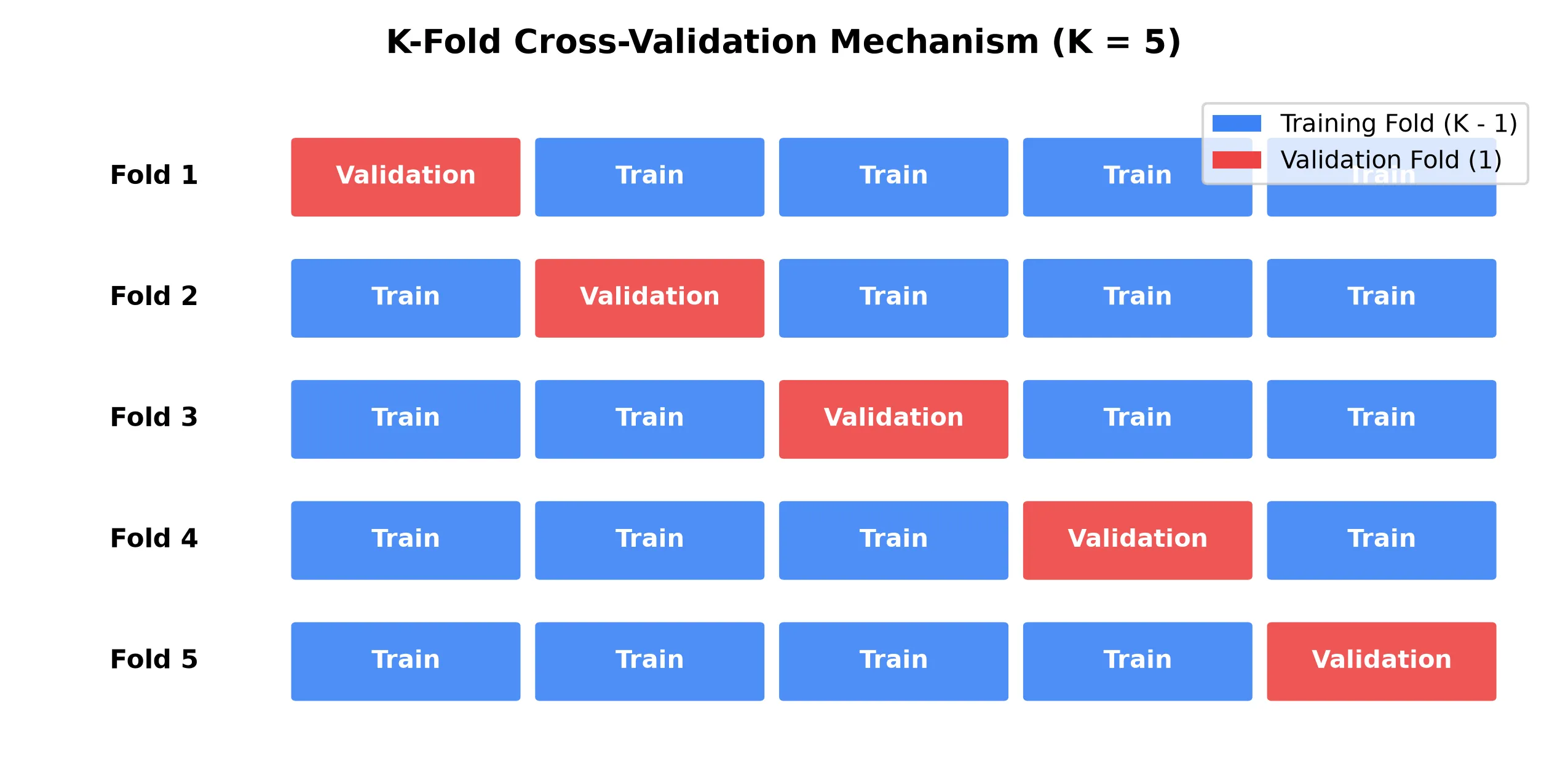
K-Fold Cross-Validation solves this problem by using all of your data for both training and validation without leaking information.
How It Works
- Split: Divide the dataset into equal parts (folds), typically or .
- Rotate: Train the model times. In each round, use 1 fold as the validation set and the remaining folds as the training set.
- Average: Calculate the average validation score across all rounds:
Code Implementation
In PyTorch, slicing and rotating the folds can be implemented in just a few lines:
def get_k_fold_data(k, i, X, y):
    fold_size = X.shape[0] // k
    start, end = i * fold_size, (i + 1) * fold_size

    X_val, y_val = X[start:end], y[start:end]
    X_train = torch.cat([X[:start], X[end:]], dim=0)
    y_train = torch.cat([y[:start], y[end:]], dim=0)

    return X_train, y_train, X_val, y_val
Then, run the loop across all folds:
models = []
all_train_losses, all_val_losses = [], []

for i in range(k):
    X_tr, y_tr, X_va, y_va = get_k_fold_data(k, i, X_train, y_train)

    # Must create a fresh model for every fold to avoid data leakage
    model = LinearRegression(num_features, lr=0.05)
    train_loss, val_loss = train(model, X_tr, y_tr, X_va, y_va, epochs=150)

    models.append(model)
    all_train_losses.append(train_loss)
    all_val_losses.append(val_loss)

avg_train_loss = sum(all_train_losses) / k
avg_val_loss = sum(all_val_losses) / k
Predicting with K-Fold
Using K models, for final predictions on the test set, pass X_test through each of the models and average their outputs:
with torch.no_grad():
    preds = [model(X_test) for model in models]
    y_test_pred = torch.stack(preds).mean(dim=0)
real_prices = torch.exp(y_test_pred).numpy()Averaging predictions across all models cancels out the individual errors of each fold model, resulting in smoother and more reliable test predictions.
8. Conclusion
- Generalization is the true goal: Low training error with high validation error means the model just memorized noise.
- Control complexity: Balance parameters, weight sizes (via weight decay), and network depth against your dataset size.
- Keep data separate: Train updates weights; Validation tunes hyperparameters; Test provides the final unbiased verdict.
- K-Fold on small datasets: It gives reliable validation without permanently sacrificing training data.