Writing CUDA code is easy, but making it run faster than a CPU is hard. Without a structured workflow, developers often optimize the wrong code or introduce subtle bugs.
This post covers APOD (Assess Parallelize Optimize Deploy), NVIDIA’s standard optimization cycle, and applies it step-by-step to Parallel Reduction.

Table of contents
Open Table of contents
- Quick Warm-up 🧠
- Part 1: The APOD Engineering Process 🔄
- Part 2: Parallel Reduction Through APOD 🧩
- 1. The Reduction Task & General Form
- 2. Assess: Sequential CPU Baseline ()
- 3. Parallelize: The Reduction Tree Concept
- 4. A Simple Single-Block Reduction Kernel (
reduceBlksKernel0) - 5. Hierarchical Reduction for Arbitrary Input Lengths 🌐
- 6. Optimize Round 1: Reducing Warp Divergence () ⚡
- Why is Slow? The Warp Divergence Limiter
- The Solution: Pack Active Threads Together
- Demystifying the Index Formula
- Kernel Implementation (
V2_compact) - Profiler Comparison: vs
- The Breakthrough: Sequential Addressing (Slide 54)
- Step-by-Step Example (4 Threads, 8 Numbers)
- Why Is Twice as Fast? Memory Coalescing
- Kernel Implementation (
V3_sequential) - Profiler Evidence: Memory Coalescing in Action
- 7. Optimize Round 2: Thread Coarsening & Grid-Stride Loops () ⚙️
- 8. Optimize Round 3: Warp Shuffle & Eliminating Barriers () 🚀
- 9. Optimize Round 4: Combining Block Results via Atomics () 🎯
- 10. Wrap-up: APOD Journey & The PCIe Reality Check 🏁
Quick Warm-up 🧠
Let’s review key concepts from the previous lecture:
Question 1: Block to Warps
A block has 256 threads. How many warps does the GPU hardware create?
Answer
Hardware groups threads into fixed 32-thread units called Warps.
Question 2: The Divergence Trap
How many warps diverge in a 256-thread block with this branch?
if (threadIdx.x % 2 == 0)
    a();
else
    b();
Answer
All 8 warps diverge (100%).
- A warp diverges if at least one thread takes a different path.
- In every warp (32 threads), 16 even threads run
a()and 16 odd threads runb(). - To fix it, group conditions in chunks of 32:
if ((threadIdx.x / 32) % 2 == 0)0 warps diverge.
Question 3: Latency Hiding
Why does an SM need many resident warps?
Answer
- Global DRAM access takes 400–800 cycles, while math takes ~4 cycles.
- When an active warp waits on DRAM (Stalled), the SM instantly swaps to another ready warp (Eligible) in 0 cycles using on-chip registers.
Part 1: The APOD Engineering Process 🔄
Professional GPU optimization is not guesswork—it is a repeatable engineering loop.
1. Why Do We Need a Process?
Developers rewriting CPU loops in CUDA often hit common traps:
- The GPU version runs slower than single-threaded CPU code.
- Days are spent optimizing a kernel that takes only 2% of total runtime.
- Fast code produces wrong results on edge-case inputs.
These stem from four mistakes:
- Guessing instead of measuring.
- Optimizing the wrong bottleneck.
- Changing too many variables at once.
- Skipping correctness checks.
2. The 4 Stages of the APOD Cycle
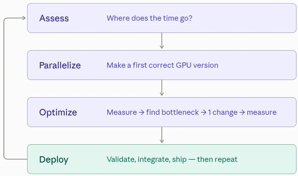 Figure 1: The cyclic APOD optimization workflow.
- Assess: Profile code, identify hotspots, and estimate possible gains.
- Parallelize: Build the simplest working GPU kernel (1 thread per output). Correctness first.
- Optimize: Measure identify limiter change one thing verify speedup.
- Deploy: Validate on production data and ship gains early ( shipped beats unfinished).
3. Assess & Amdahl’s Law
Before writing CUDA, evaluate the theoretical ceiling. Amdahl’s Law states that program speedup is strictly limited by its serial (unparallelized) fraction:
- : Parallelizable fraction of execution time.
- : Serial fraction (file I/O, sequential CPU work).
- : Speedup of the parallelized portion.
| Parallel Fraction () | Speedup () | Speedup () | Infinite Cores () |
|---|---|---|---|
| 50% | |||
| 90% | |||
| 99% |
The 40× Trap: If an image pipeline spends 80s in filter() and 20s in file I/O (total 100s), speeding up filter() by on GPU reduces its time to 2s. The new total time is , giving only a application speedup.
4. Profiling Cheatsheet & Key Metrics 💻
Never guess—use standard profiling tools to answer specific questions:
Measuring Accurate Time (cudaEvent)
cudaEvent_t start, stop;
cudaEventCreate(&start); cudaEventCreate(&stop);

// Warm-up launch (driver setup overhead)
kernel<<<grid, block>>>(d_in, d_out, n);

cudaEventRecord(start);
kernel<<<grid, block>>>(d_in, d_out, n);
cudaEventRecord(stop);
cudaEventSynchronize(stop);

float ms = 0.0f;
cudaEventElapsedTime(&ms, start, stop);
Application vs Kernel Profiling CLI
# 1. Nsight Systems: Whole-program timeline (CPU, PCIe copies, GPU kernels)
nsys profile --stats=true -o app_report ./my_app
nsys stats app_report.nsys-rep

# 2. Nsight Compute: Single-kernel hardware diagnostics
ncu --section SpeedOfLight --section Occupancy --section WarpStateStats -k regex:myKernel -c 1 ./my_app
Essential Metrics & Formulas
| Question | Hardware Metric | Target |
|---|---|---|
| Are threads diverging? | smsp__thread_inst_executed_per_inst_executed.ratio | 32.0 (no divergence) |
| Are branches uniform? | smsp__sass_average_branch_targets_threads_uniform.pct | 100% |
| Is the SM occupied? | sm__warps_active.avg.pct_of_peak_sustained_active | 75–100% |
| DRAM bandwidth achieved? | dram__bytes_read.sum.per_second | Compare to GPU peak (320 GB/s on T4) |
5. The APOD Optimization Log 📝
Track every optimization round with one hypothesis and one change at a time:
| Version | Change (Only One!) | Hypothesis | Time (ms) | Speedup vs CPU | Effective Bandwidth | Decision |
|---|---|---|---|---|---|---|
| CPU Baseline | Single-threaded reference | 47.2 ms | 1.4 GB/s | Ground Truth | ||
| Basic Tree Reduction | First parallel version | 1.81 ms | 37.1 GB/s | Baseline GPU | ||
| Compact Active Threads | Eliminate warp divergence | 1.67 ms | 40.1 GB/s | Keep | ||
| Sequential Addressing | Enable coalesced memory reads | 0.89 ms | 75.4 GB/s | Keep (2× gain) | ||
| Thread Coarsening | Grid-stride loop + registers | 0.325 ms | 206.7 GB/s | Keep (3× gain) | ||
| Warp Shuffle | Register exchange via __shfl_down_sync | 0.324 ms | 206.8 GB/s | Keep | ||
| Block Atomics | GPU atomicAdd across blocks | 0.330 ms | 203.6 GB/s | Keep |
Part 2: Parallel Reduction Through APOD 🧩
Now we apply APOD to optimize array summation across multiple rounds.
1. The Reduction Task & General Form
A Reduction combines an array of elements into a single scalar value using an associative binary operator:
- Sum: (identity: , operator: )
- Product: (identity: , operator: )
- Min / Max: or (identity: )
A reduction can only run in parallel if the operator is associative: .
2. Assess: Sequential CPU Baseline ()
int reduceOnHost(int *in, int n) {
    int s = in[0];
    for (int i = 1; i < n; i++) {
        s += in[i];
    }
    return s;
}- Complexity: steps time, additions work.
- Dataset: ints ().
- CPU time (): .
- Hardware Speed-of-Light target (Tesla T4 peak 320 GB/s):
Our optimization goal is to push kernel execution toward this ceiling.
3. Parallelize: The Reduction Tree Concept
Instead of adding numbers sequentially, threads pair up elements in a binary tree:
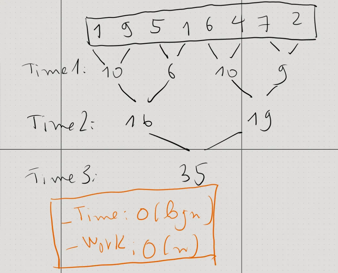 Figure 2: Parallel reduction tree pairwise summation across time steps.
The Numbers Behind the Tree
- Total Work: (Work-efficient).
- Execution Steps: (For , only 20 steps vs 1,000,000 on CPU).
- Peak Resource Demand: at Step 1.
- Average Parallelism:
When is the Tree Allowed?
The parallel tree changes the evaluation order:
- Sequential:
- Parallel:
The operation must satisfy:
-
Associative:
-
Commutative: (required when reordering operands across threads)
-
Allowed: Integer , , , , AND, OR, XOR.
-
Disallowed: Subtraction, division (non-associative).
-
Note on Floats: Floating-point addition is not strictly associative due to rounding, so GPU and CPU sums can differ slightly.
Parallel Reduction in Real Life
- Sports & Tournaments: Single-elimination brackets to find a tournament winner ( reduction).
- Big Data & MapReduce: Google and Hadoop partition massive datasets into chunks and use reduction trees to compute global sums, word counts, and aggregate logs.
- Machine Learning & Vision: Batch normalization, loss reduction (MSE, cross-entropy), dot products, vector norms, and image histograms.
The Resource Inefficiency Bottleneck: While Step 1 needs 500,000 threads, subsequent steps cut active threads in half each time. In later steps, over 90% of threads sit idle while still reserving registers and SM slots.
4. A Simple Single-Block Reduction Kernel (reduceBlksKernel0)
Before scaling up to millions of elements across multiple blocks, let’s examine the baseline implementation for a single block (Slide 34–35).
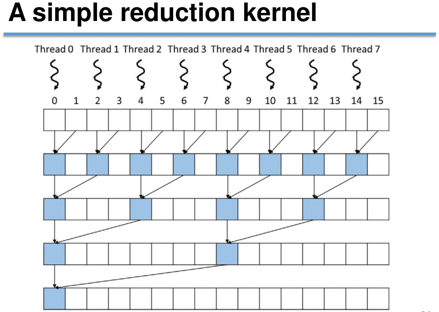 Figure 3: Thread-to-data mapping in a single-block reduction kernel across stride doubling steps.
Implementation
__global__ void reduceBlksKernel0(int* in, int* out, int n) {
    int i = 2 * threadIdx.x;

    for (int stride = 1; stride <= blockDim.x; stride *= 2) {
        if (threadIdx.x % stride == 0)
            in[i] += in[i + stride];
        __syncthreads();
    }

    if (threadIdx.x == 0)
        *out = in[0];
}
Step-by-Step Breakdown
- Thread-to-Data Mapping (
i = 2 * threadIdx.x):- Each thread initially manages two contiguous elements.
- Thread 0 starts at index 0, Thread 1 at index 2, Thread 2 at index 4, etc.
- Iterative Stride Doubling (
stride *= 2):- At
stride = 1: all threads are active (tid % 1 == 0), pairing indices . - At
stride = 2: only even threads participate (tid % 2 == 0), pairing . - At
stride = 4: only threads divisible by 4 participate, pairing . - After steps, the block’s sum accumulates at
in[0].
- At
- Barrier Synchronization (
__syncthreads()):- Forces all threads in the block to finish reading and writing their pair before advancing to the next stride.
- Prevents data races where a fast thread in step reads an index before a slower thread in step writes to it.
- Final Output (
threadIdx.x == 0):- Thread 0 writes the reduced block result
in[0]to*out.
- Thread 0 writes the reduced block result
Critical Limitations
Why this kernel cannot scale directly to arbitrary input sizes:
- Block Boundary Constraint:
__syncthreads()synchronizes threads within the same block only. Because a CUDA block has a hardware ceiling of 1024 threads, this kernel can reduce at most elements. - Severe Warp Divergence: The condition
threadIdx.x % stride == 0causes thread divergence within warps. Even if only 1 thread in a warp of 32 is active, the entire warp must still be scheduled.
To handle arbitrary array lengths (), we must extend this into Hierarchical Multi-Block Reduction.
5. Hierarchical Reduction for Arbitrary Input Lengths 🌐
In real-world applications, arrays contain millions of elements (). Because __syncthreads() cannot synchronize across different blocks, we solve this with Hierarchical Reduction:
- Partition: Divide the array into independent chunks, assigning one chunk of elements to each block.
- Local Block Reduction: Each block computes its own partial sum using tree reduction.
- Global Accumulation: Combine the partial sums into the final result.
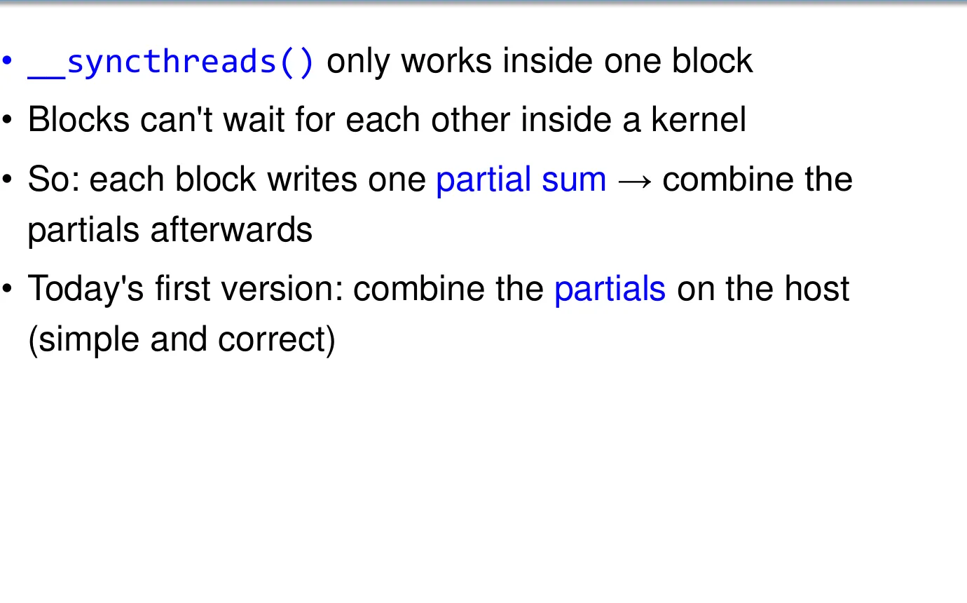 Figure 4: Hierarchical reduction partitioning input into blocks to produce partial sums.
Kernel Implementation (V1_naive)
__global__ void reduceV1_naive(int *in, int *partial, int n) {
    // Starting index of this block (each block handles 2 * blockDim.x elements)
    int start = blockIdx.x * 2 * blockDim.x;
    int i = start + 2 * threadIdx.x;

    // Tree reduction inside the block
    for (int stride = 1; stride <= blockDim.x; stride *= 2) {
        if (threadIdx.x % stride == 0) {
            // Guard boundary for arbitrary array sizes
            if (i + stride < n) {
                in[i] += in[i + stride];
            }
        }
        __syncthreads();
    }

    // Thread 0 writes the block's partial sum
    if (threadIdx.x == 0) {
        partial[blockIdx.x] = in[start];
    }
}
Host-Side Launch Configuration
To cover arbitrary array lengths , calculate gridSize using ceiling division:
dim3 blockSize(512);
dim3 gridSize((n + 2 * blockSize.x - 1) / (2 * blockSize.x));

// Launch kernel to compute partial sums per block
reduceV1_naive<<<gridSize, blockSize>>>(d_in, d_partial, n);

// Copy partial sums back to Host and accumulate sequentially on CPU
cudaMemcpy(h_partial, d_partial, gridSize.x * sizeof(int), cudaMemcpyDeviceToHost);
int total_sum = 0;
for (int b = 0; b < gridSize.x; b++) {
    total_sum += h_partial[b];
}Pitfall: In-Place Reduction Destroys Input Data!
in[i] += in[i + stride] modifies the input array in-place. If benchmarking execution time across multiple iterations, you must restore the original input array (cudaMemcpy) before each timed run, otherwise subsequent runs will sum already-reduced values!
6. Optimize Round 1: Reducing Warp Divergence () ⚡
Why is Slow? The Warp Divergence Limiter
In , the condition if (threadIdx.x % stride == 0) causes severe warp divergence.
Consider a block of 256 threads (8 warps):
stride = 1: All 256 threads are active 0 diverged warps.stride = 2: Threads withtid % 2 == 0run (128 threads). Every warp has 16 active and 16 idle threads All 8 warps diverge!stride = 64: Only 4 threads run (tid = 0, 64, 128, 192). They land in Warps 0, 2, 4, 6 4 warps diverge (each warp runs for only 1 active thread, wasting 31 slots).- Across all iterations, triggers 47 diverged warp instances. Moreover, the modulo operator (
%) is an expensive division instruction on GPU.
The Solution: Pack Active Threads Together
Instead of scattering active threads across all warps, compacts all working threads into the first contiguous threads (threadIdx.x < threshold).
This ensures:
- Active warps run at 100% capacity (no divergence inside).
- Inactive warps have 0 active threads the hardware warp scheduler skips them entirely with zero cost!
V1 (Scattered):  [X . X . X . X .]   -> Warp suffers 50% divergence
V2 (Compacted):  [X X X X . . . .]   -> Warp 0 runs at 100%, Warp 1 disabled
Demystifying the Index Formula
To let adjacent threads process numbers spread across the block, uses:
Why ? It acts as a stride multiplier so that lower-index threads jump to the correct data pairs:
stride = 1: Step is . Thread 0 pairs , Thread 1 pairs , Thread 2 pairs .stride = 2: Step is . Thread 0 pairs , Thread 1 pairs .stride = 4: Step is . Thread 0 pairs .
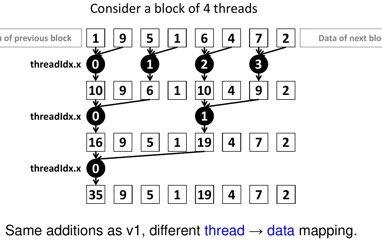 Figure 5: V2 thread-to-data mapping packing active threads into the front.
Threads do all the work, while warps with higher thread IDs stay completely asleep.
Kernel Implementation (V2_compact)
__global__ void reduceV2_compact(int *in, int *partial, int n) {
    int start = blockIdx.x * 2 * blockDim.x;

    for (int stride = 1; stride <= blockDim.x; stride *= 2) {
        // Stride multiplier lets contiguous threads reach distant elements
        int i = start + threadIdx.x * 2 * stride;

        // Condition packs all active threads into the front
        if (threadIdx.x < blockDim.x / stride) {
            if (i + stride < n) {
                in[i] += in[i + stride];
            }
        }
        __syncthreads();
    }

    if (threadIdx.x == 0) {
        partial[blockIdx.x] = in[start];
    }
}
Profiler Comparison: vs
Using Nsight Compute (ncu) to measure active threads per warp instruction:
| Kernel Version | Active Threads / Warp Inst | Warp Efficiency | Wasted Slots |
|---|---|---|---|
| (Naive) | 28.75 / 32 | ||
| (Compacted) | 31.20 / 32 |
Why is only slightly faster?
In our benchmark, execution time improves from 1.81 ms () to 1.67 ms (). While warp efficiency jumped to 97.5%, the speedup is modest. Calculating i adds arithmetic overhead, but more critically, adjacent active threads access data spaced far apart (2 * stride), causing non-coalesced memory loads (and shared memory bank conflicts). This brings us to !
The Breakthrough: Sequential Addressing (Slide 54)
In , active threads were grouped together, but they still read numbers spaced far apart. This caused uncoalesced memory access — the GPU fetched 32 bytes from memory just to use one 4-byte number!
solves this by reversing the reduction tree:
- Start with a large stride:
stride = blockDim.x(half the block’s data). - Cut the stride in half each round:
stride /= 2until it reaches 1. - Each thread simply accesses its own neighboring index:
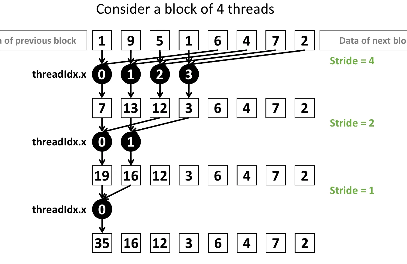 Figure 6: Sequential addressing reverses the stride so adjacent threads read adjacent memory words.
Step-by-Step Example (4 Threads, 8 Numbers)
Consider the example from Slide 54 with array [1, 9, 5, 1, 6, 4, 7, 2]:
-
Round 1 (
stride = 4): Threads 0, 1, 2, 3 are active (threadIdx.x < 4). Each thread pairs with element :- Thread 0:
in[0] += in[4] - Thread 1:
in[1] += in[5] - Thread 2:
in[2] += in[6] - Thread 3:
in[3] += in[7] - Array becomes:
[ 7, 13, 12, 3 | 6, 4, 7, 2 ]
- Thread 0:
-
Round 2 (
stride = 2): Only Threads 0 and 1 are active (threadIdx.x < 2). Pair with element :- Thread 0:
in[0] += in[2] - Thread 1:
in[1] += in[3] - Array becomes:
[ 19, 16 | 12, 3 | 6, 4, 7, 2 ]
- Thread 0:
-
Round 3 (
stride = 1): Only Thread 0 is active (threadIdx.x < 1). Pair with element :- Thread 0:
in[0] += in[1] - Final block sum:
in[start] = 35!
- Thread 0:
Why Is Twice as Fast? Memory Coalescing
- In , adjacent threads read numbers spaced far apart wasted bandwidth.
- In , Threads 0, 1, 2, 3 read numbers side-by-side in memory the GPU hardware loads all of them in one single 32-byte memory transaction (Coalescing)!
Kernel Implementation (V3_sequential)
__global__ void reduceBlksKernel3(int *in, int *out, int n) {
    int start = blockIdx.x * 2 * blockDim.x;
    int i = start + threadIdx.x;

    // Reverse stride from half-block down to 1
    for (int stride = blockDim.x; stride > 0; stride /= 2) {
        if (threadIdx.x < stride) {
            if (i + stride < n) {
                in[i] += in[i + stride];
            }
        }
        __syncthreads();
    }

    if (threadIdx.x == 0) {
        atomicAdd(out, in[start]);
    }
}
Profiler Evidence: Memory Coalescing in Action
Comparing the hardware memory transactions in Nsight Compute:
ncu --metrics l1tex__t_requests_pipe_lsu_mem_global_op_ld.sum,\
l1tex__t_sectors_pipe_lsu_mem_global_op_ld.sum \
-k regex:"reduce.*" ./reduce 256| Kernel Version | Load Requests | Sectors Fetched (32B) | Global Memory Traffic | Execution Time |
|---|---|---|---|---|
| (Naive) | 227,335 | 1,046,535 | High | 1.81 ms |
| (Compacted) | 83,975 | 1,046,535 | High (identical to ) | 1.67 ms |
| (Sequential) | 83,975 | 272,391 | 3.8× Less Traffic! | 0.85 ms (2× faster!) |
Key Insight: fixed warp divergence but fetched the exact same memory sectors as because adjacent threads were reading far-apart addresses. fixed the memory layout: consecutive threads read consecutive bytes, cutting bus traffic by and doubling execution speed!
7. Optimize Round 2: Thread Coarsening & Grid-Stride Loops () ⚙️
Assessing : Too Many Threads Doing Too Little
While achieved an impressive speedup over CPU, a critical resource inefficiency remains:
- Massive thread count: 1 thread per 2 elements means launching 8 million threads (32,768 blocks) for .
- Idle threads: After step 1, 50% of threads are idle. After step 3, 87.5% of threads are idle.
- High barrier overhead: Each block executes 9 synchronization barriers (
__syncthreads()) just to reduce 512 elements. - Host burden: The GPU produces 32,768 partial sums that must be transferred and summed.
The Coarsening Concept: Do More Work in Registers
Instead of creating millions of threads that die after one step, Thread Coarsening gives each thread multiple elements to sum locally before entering the tree:
- Step 1 (Sequential Accumulation): Each thread loops over multiple elements spaced by the grid stride and accumulates the sum in a private register variable.
- Step 2 (Block Tree Reduction): Once the data is condensed, threads run the tree reduction on just one value per thread.
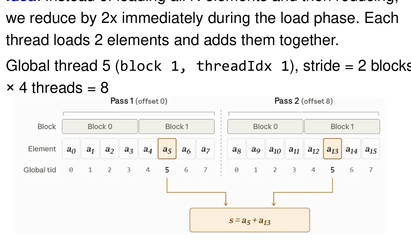 Figure 7: Thread coarsening aggregates multiple elements sequentially in private registers.
Accumulating in private registers requires zero synchronization barriers and zero global memory writes.
The Grid-Stride Loop Pattern
Rather than launching 32,768 blocks, we launch just enough blocks to saturate all Streaming Multiprocessors (SMs) on the GPU (e.g., blocks of 256 threads on Tesla T4):
int gid = blockIdx.x * blockDim.x + threadIdx.x;
int totalThreads = gridDim.x * blockDim.x;

int sum = 0;
// Each thread sums elements spaced by the entire grid width
for (int k = gid; k < n; k += totalThreads) {
    sum += in[k];
}- Scalable: Runs safely for arbitrary array sizes with any grid configuration.
- Coalesced: In every iteration, thread and thread access contiguous memory addresses.
- Hardware-friendly: Replaces 32,768 blocks with 160 persistent blocks.
Kernel Implementation (V4_coarsened)
__global__ void reduceV4_coarsened(int *in, int *out, int n) {
    extern __shared__ int sdata[];

    int gid = blockIdx.x * blockDim.x + threadIdx.x;
    int totalThreads = gridDim.x * blockDim.x;

    // 1. Thread coarsening: accumulate multiple elements into a register
    int sum = 0;
    for (int k = gid; k < n; k += totalThreads) {
        sum += in[k];
    }

    sdata[threadIdx.x] = sum;
    __syncthreads();

    // 2. Sequential addressing tree within shared memory
    for (int stride = blockDim.x / 2; stride > 0; stride /= 2) {
        if (threadIdx.x < stride) {
            sdata[threadIdx.x] += sdata[threadIdx.x + stride];
        }
        __syncthreads();
    }

    // 3. Block leader writes result
    if (threadIdx.x == 0) {
        atomicAdd(out, sdata[0]);
    }
}
Benchmark Result: Execution time plunges from down to ! Throughput skyrockets to ( speedup over CPU).
8. Optimize Round 3: Warp Shuffle & Eliminating Barriers () 🚀
The Final Barrier Bottleneck
In the final 5 steps of the block tree reduction (when stride < 32), all active threads reside inside Warp 0 (threads through ).
Yet, standard shared memory code still executes:
- Multiple reads and writes to shared memory.
__syncthreads()barrier instructions at every single step!
Because threads in a warp execute synchronously in lockstep, barriers within a single warp are completely redundant.
The Solution: Warp Shuffle (__shfl_down_sync)
CUDA provides warp shuffle instructions that allow threads inside the same warp to read each other’s register values directly across the SM crossbar network:
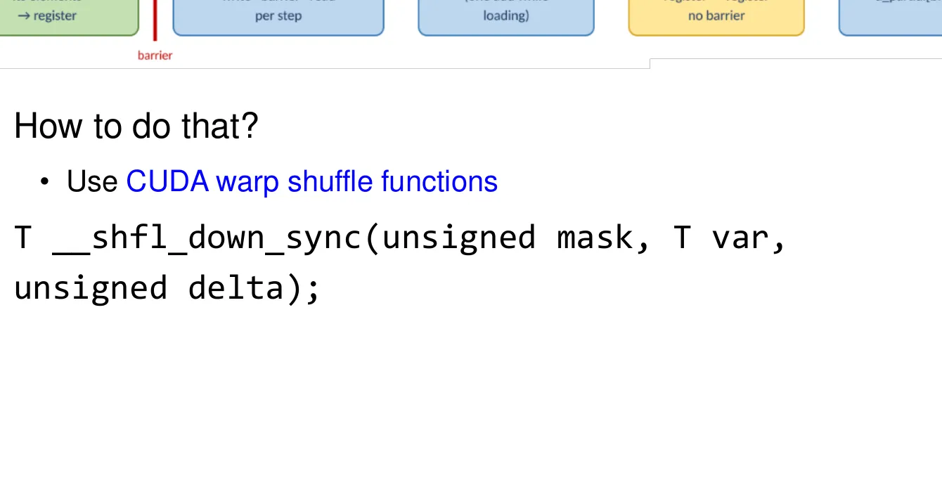 Figure 8: Intra-warp register-to-register value exchange via __shfl_down_sync.
- Zero Memory Overhead: Values travel directly from register to register without touching shared or global memory.
- Zero Barrier Stalls: No
__syncthreads()needed!
inline __device__ int warpReduceSum(int val) {
    for (int offset = 16; offset > 0; offset /= 2) {
        val += __shfl_down_sync(0xffffffff, val, offset);
    }
    return val;
}
Replacing shared memory reduction in Warp 0 with warpReduceSum() shaves off remaining latency, achieving and .
9. Optimize Round 4: Combining Block Results via Atomics () 🎯
How Should We Combine Block Partials?
Once each block finishes reducing its portion, how do we aggregate the final scalar result?
| Option | Approach | Trade-off / Cost |
|---|---|---|
| Option A: Host Finish | Copy partials back to CPU and sum in a loop | High PCIe latency, slow serial CPU loop (–) |
| Option B: Second Kernel | Launch another reduction kernel on the partial array | Kernel launch overhead |
| Option C: GPU Atomic Add | Block leader threads add directly into single global memory address | Hardware-serialized atomic contention |
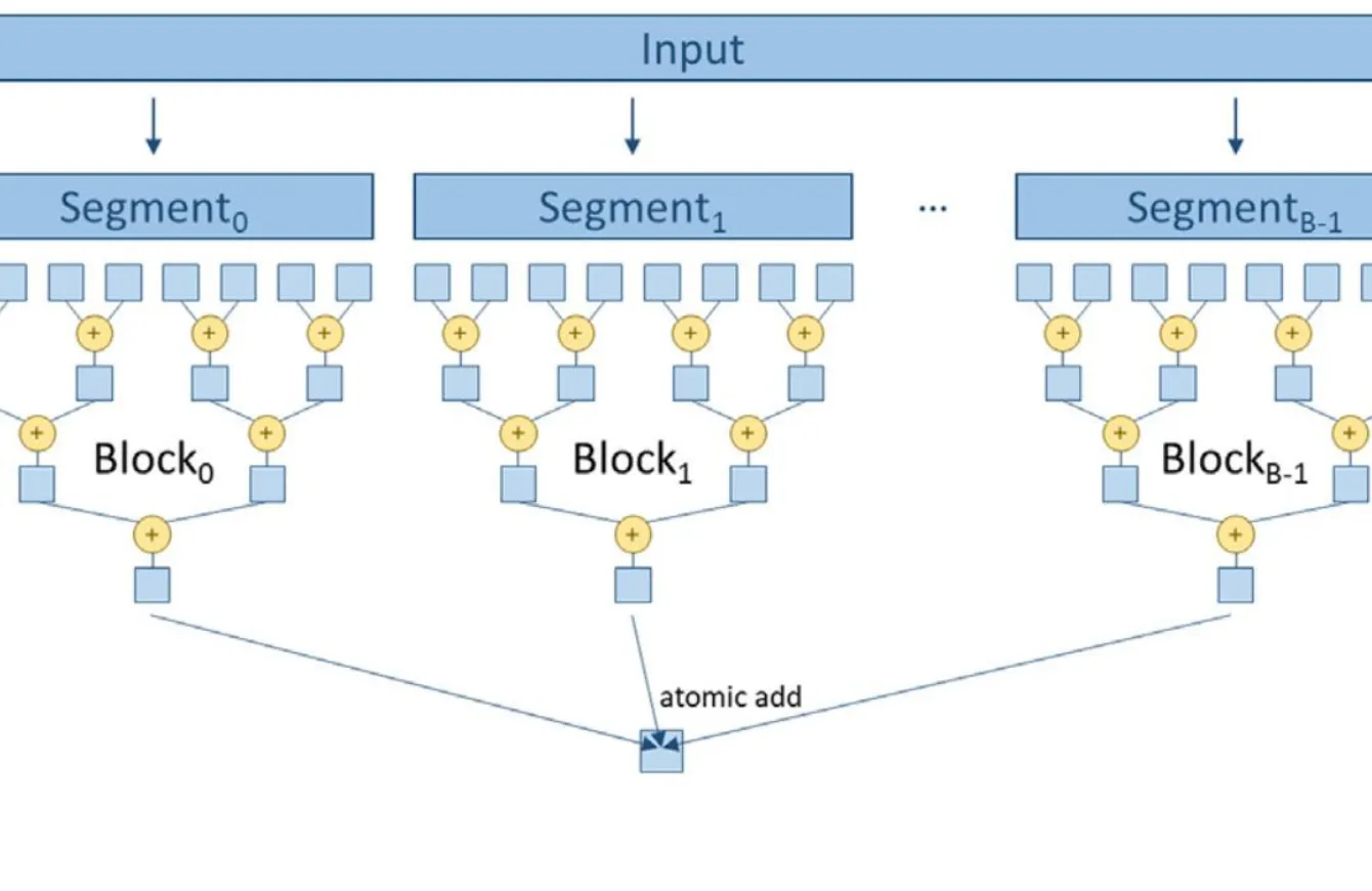 Figure 9: Block leader threads atomically update a single global memory scalar.
Why Atomics Win With Coarsening
When we had 32,768 blocks in , having 32,768 blocks write to one address caused heavy memory serialization.
However, with Thread Coarsening (), we only launch 160 blocks! Serializing 160 atomic additions takes less than , completely obliterating the milliseconds spent copying partial arrays to the host:
if (threadIdx.x == 0) {
    atomicAdd(out, sdata[0]); // Only 160 atomic updates across the whole GPU!
}Data Race Warning:
Never permit multiple threads inside the same block to write to the global accumulator simultaneously. Only designated leader threads (threadIdx.x == 0) should invoke atomicAdd.
10. Wrap-up: APOD Journey & The PCIe Reality Check 🏁
Comprehensive Optimization Scorecard (Tesla T4)
Benchmark results for reducing integers ( of data) on NVIDIA Tesla T4 ( peak bandwidth):
| Kernel Version | Optimization Strategy | Bottleneck Removed | Time (ms) | Effective BW | Speedup |
|---|---|---|---|---|---|
| Host CPU | Single-core C++ sequential loop | — | 43.76 ms | 1.5 GB/s | (ref) |
| Naive GPU | Basic parallel reduction tree | Serial CPU loop | 1.635 ms | 41.0 GB/s | |
| Compact Threads | Contiguous active thread indexing | Warp divergence | 1.621 ms | 41.4 GB/s | |
| Sequential Addr | Reversed stride + contiguous layout | Strided uncoalesced memory | 0.849 ms | 79.0 GB/s | |
| Coarsened | Grid-stride loop + registers | Idle threads & barrier stalls | 0.325 ms | 206.7 GB/s | |
| Warp Shuffle | __shfl_down_sync register exchange | Shared memory & warp barriers | 0.324 ms | 206.8 GB/s | |
| Atomics | Block-level atomicAdd | Host partial collection | 0.330 ms | 203.6 GB/s | |
| NVIDIA CUB | cub::DeviceReduce::Sum | Industrial reference | 0.394 ms | 170.4 GB/s |
Approaching the Speed-of-Light (SOL)
With , our custom CUDA kernel achieved:
This represents of the theoretical physical ceiling () and comfortably outpaces NVIDIA’s heavily tuned CUB library () for this workload size.
The PCIe Reality Check: Amdahl’s Law Strikes Back!
Before celebrating a speedup, examine the end-to-end wall clock time:
[ CPU Sequential Sum ] ======================================> 43.7 ms

[ GPU Execution Flow ]
|-- PCIe H2D Copy (14.8 ms) --|-- Kernel (0.32 ms) --|-- D2H Copy (0.01 ms) --|
Total GPU Wall-Clock = 15.1 ms| Component | Time (ms) | Percentage of Total Time |
|---|---|---|
| PCIe Transfer (Host Device) | 14.8 ms | 97.9% |
| Optimized GPU Kernel () | 0.32 ms | 2.1% |
| Total GPU End-to-End | 15.1 ms | 100.0% |
The Real-World Lesson: While the kernel itself is faster than the CPU, the overall application is only faster ( vs ) because PCIe transfer consumes of the total runtime! To unlock the full power of GPUs:
- Keep data on device: Chain multiple GPU operations together so data stays in VRAM.
- Overlap transfers: Use CUDA Streams and Pinned (
cudaHostAlloc) memory to overlap compute with PCIe copies.
Summary Checklist: The APOD Engineering Takeaway
- Never guess—profile first: Use
nsysfor system-level timelines andncufor warp-level micro-architecture bottlenecks. - Eliminate Warp Divergence: Ensure warps are either 100% active or 100% idle.
- Coalesce Memory Accesses: Ensure adjacent threads access adjacent 4-byte words to utilize all 32 bytes of every memory sector.
- Coarsen Threads: Don’t launch millions of short-lived threads; use grid-stride loops to accumulate values locally in registers with zero synchronization cost.
- Leverage Warp-Level Primitives: Replace intra-warp shared memory and
__syncthreads()with fast register shuffles (__shfl_down_sync). - Aggregate with Atomics: When thread count is kept compact, GPU
atomicAddis far faster than offloading aggregation to the CPU.